

In the previous posts, we laid the mathematical foundation necessary for implementing the error state kalman filter. In this post, we’ll provide the Matlab implementation for performing sensor fusion between accelerometer and gyroscope data using the math developed earlier.
Lets recapitulate our notation and definition of various quantities as introduced in the previous post.
-
 for angular velocity
 for acceleration
 for the gyro bias
 for the accel bias
- subscript m to denote measured quantities and hat to denote estimated quantities
- True values appear without annotation.
The measured value of the gyro is the true value corrupted with the gyro bias and random noise. Therefore,

Here the rate noise  is assumed to be gaussian white noise with characteristics
![E[\boldsymbol{n_r}] = 0_{3\times1}, E[\boldsymbol{n_r} (t+\tau) \boldsymbol{n_r^T}(t)] = \boldsymbol{N_r}\delta(\tau)](https://www.telesens.co/wp-content/ql-cache/quicklatex.com-fb7611c58a2e60273760f32824b8968d_l3.png "Rendered by QuickLaTeX.com")
The gyro bias is non-static (otherwise it need not be estimated) and modeled as a random walk process:
![E[\boldsymbol{n_b}] = 0_{3\times1}, E[\boldsymbol{n_b} (t+\tau) \boldsymbol{n_b^T}(t)] = \boldsymbol{N_b}\delta(\tau)](https://www.telesens.co/wp-content/ql-cache/quicklatex.com-e67f64eff7f6124978e39f721e71aa70_l3.png "Rendered by QuickLaTeX.com")
We’ll also assume that the associated covariance matrices are diagonal:

and

The estimated angular rate is the difference between the measured rate and our estimate of the gyro bias


Here,  is the gyro bias error.
Our state vector consists of the error in the orientation and the error in the gyro bias.
![\bf{x} = [\boldsymbol{\delta{\theta}}, \boldsymbol{\delta{\omega_b}}]](https://www.telesens.co/wp-content/ql-cache/quicklatex.com-5f1b452dec5a82c0046f3cb2496afcff_l3.png "Rendered by QuickLaTeX.com")
The error in orientation is defined as the vector of small rotations that aligns the estimated rotation with the true rotation. The corresponding error quaternion is approximated by:

We derived the state transition matrix  in the last post. This matrix is given by:
![F = \begin{bmatrix}-[\hat{\phi}]_\times & I_{3\times3}\delta{t} \\ 0_{3\times3} & 0_{3\times3}\end{bmatrix}](https://www.telesens.co/wp-content/ql-cache/quicklatex.com-0226f8c69c940bfd583e7586f883b1b6_l3.png "Rendered by QuickLaTeX.com")
Where
![[\hat{\phi}]_\times = [\hat{\omega}]_\times \delta{t}](https://www.telesens.co/wp-content/ql-cache/quicklatex.com-04e7f0f79eb2788f06a6bc2f562f5f59_l3.png "Rendered by QuickLaTeX.com")
In a typical Kalman filter implementation, the state is updated every time step. Our implementation uses a different configuration of the Kalman filter called the feedback configuration. In this configuration, when the error state variables are updated as a result of processing a measurement, the updates are applied directly to the system state (in this case, the orientation and gyro bias). Thus, at each time step, we set the error state to be 0. For more information about the feedback configuration, see chapter 6 of 1.
We do update the error state covariance in every time step. This is done in the regular way:

Here  denotes the time step index.
Now let’s look at the measurement update step. We’ll first use the accelerometer to provide measurement updates and then add image based measurements. The accelerometer readings can be used as a measurement source as they provide direct measurement of the orientation and don’t suffer from drift (although they can have a bias, which can also be estimated). As the name suggests, the accelerometer measures the total acceleration in the body coordinate system. For a body at rest or moving a constant velocity, the accelerometer will measure the reaction to the force of gravity. Let’s denote the reaction to acceleration due to gravity by the vector ![[0, 0, g]](https://www.telesens.co/wp-content/ql-cache/quicklatex.com-a3c53d4bac09535c0575c324310de779_l3.png "Rendered by QuickLaTeX.com") and the current orientation of the body frame wrt the global frame by
and the current orientation of the body frame wrt the global frame by  . Then, the accelerometer readings are given as:

While formulating the measurement update equation, we need to express the measurement residual (denoted by  ), the difference between the estimated and the true value of the measurements as a linear function of the state vector.
In order to formulate the residual, we need to transform back to the global reference frame. This can be done by post multiplying by  . Note that don’t know the true DCM , only its estimated value. Therefore multiplying by
  is the best we can do.


Now recall from the previous post that ![C = \hat{C} + \hat{C}[\delta{\theta}]_\times](https://www.telesens.co/wp-content/ql-cache/quicklatex.com-179ff668dd5e4aa79e31be8616aaabb6_l3.png "Rendered by QuickLaTeX.com") . Also, since
. Also, since ![[\delta{\theta}]_\times](https://www.telesens.co/wp-content/ql-cache/quicklatex.com-19ea934b2e31e7ba903b36da835825cb_l3.png "Rendered by QuickLaTeX.com") is skew symmetric,
is skew symmetric, ![[\delta{\theta}]_\times^T](https://www.telesens.co/wp-content/ql-cache/quicklatex.com-1c0012034deac153bbf484cbe543f0f8_l3.png "Rendered by QuickLaTeX.com") =
= ![-[\delta{\theta}]_\times](https://www.telesens.co/wp-content/ql-cache/quicklatex.com-bb9acb7f0f5787e0b6cf6c062cb07b0a_l3.png "Rendered by QuickLaTeX.com") . Applying these properties,
. Applying these properties,
![\boldsymbol{z} = C[\delta{\theta}]_\times \hat{C}^T\boldsymbol{g}](https://www.telesens.co/wp-content/ql-cache/quicklatex.com-d070817748b2cc92a61b1f129f56aa70_l3.png "Rendered by QuickLaTeX.com")
Now, applying the approximation that for small orientation errors,  ,
,
![\boldsymbol{z} \approx \hat{C}[\delta{\theta}]_\times \hat{C}^T\boldsymbol{g}](https://www.telesens.co/wp-content/ql-cache/quicklatex.com-2ef19f92ae7acebe62bd6e69740f8df2_l3.png "Rendered by QuickLaTeX.com")
From equation 49 in 1, ![[Ca]_\times= C[a]_\times C^T](https://www.telesens.co/wp-content/ql-cache/quicklatex.com-900361d0a0b05826bf79947995591d50_l3.png "Rendered by QuickLaTeX.com") . Therefore,
. Therefore,
![\boldsymbol{z} = [\hat{C}\boldsymbol{\delta{\theta}}]_\times\boldsymbol{g}](https://www.telesens.co/wp-content/ql-cache/quicklatex.com-4c72c96c749f15a2395eae6add5ceb7c_l3.png "Rendered by QuickLaTeX.com")
From equation 39 in 1, ![[a]_\times\boldsymbol{b} = -[b]_\times\boldsymbol{a}](https://www.telesens.co/wp-content/ql-cache/quicklatex.com-0912dd31551b6b1384fd1cca4e651945_l3.png "Rendered by QuickLaTeX.com") . Therefore,
. Therefore,
(1) ![\begin{equation*} \boldsymbol{z} = -[g]_\times \hat{C}\boldsymbol{\delta{\theta}}\end{equation*}](https://www.telesens.co/wp-content/ql-cache/quicklatex.com-a279e25490c292935d600c6b10960980_l3.png "Rendered by QuickLaTeX.com")
The accelerometer doesn’t provide direct observability on the bias, and therefore the term corresponding to the bias error part in the state vector is 0. The complete  matrix is given by:
(2) ![\begin{equation*} H_{accel} = \begin{bmatrix} -[g]_\times \hat{C} & 0 \end{bmatrix} \end{equation*}](https://www.telesens.co/wp-content/ql-cache/quicklatex.com-cb157027be311645c2f373a663edaead_l3.png "Rendered by QuickLaTeX.com")
Setting the Covariance Matrices
A major benefit of the Kalman filter is that not only does it perform the most optimal state estimation (under its operating assumptions) but it also provides an estimate of the state covariance matrix, allowing us to put a confidence interval around the estimated state variables. To do this, the filter takes as input three covariance matrices:
 : The initial value of the state covariance matrix. This can be set to suitable values reflecting our initial uncertainty in measuring the initial state. It only effects the transient behaviour of the filter, not the final (converged) value of the covariance matrix.
 : This is measurement uncertainty matrix, reflecting the uncertainty induced due to various errors in the measurements.
 : This is the process noise covariance, and reflects the amount of uncertainty being added in each step of the Kalman filter update. This matrix is usually the trickiest to estimate.
A common method used to quantify various noise sources in inertial sensor data is called AllanVariance. The basic idea is to compute the variance between clusters of overlapping data with different stride lengths.
The basic idea is that short term sources of noise such as random walk and quantification errors appear over smaller values of  and average out over larger samples. Long term error sources such as gyro bias random walk appears over larger samples. Thus, by examining the slope of the plot of variance against stride length, different source of error can be visualized and quantified. I however found several aspects of Allan Variance charts hard to understand. For example, it is not clear to me why the gyro random walk noise appears on the chart with a gradient of -0.5.
I therefore tried a different method to obtain good values for the elements of the covariance matrix. I collected data from the MPU6050 unit (integrated MEMS gyro+accel from Invensense) with the unit at rest and fit a Gaussian distribution to the data using the fitdist function in Matlab. The code is shown below:
|
1 2 3 4 5 6 7 8 9 10 11 12 13 14 15 16 17 18 19 20 21 22 23 24 25 26 27 28 |
DEGTORAD = pi/180; fs = 100; ts = 1/fs; % Scale raw gyro readings to obtain data in rad/sec scaled_data_gyro = raw_data(:, 2:4)./GYRO_SCALE_FACTOR; scaled_data_gyro_rad = scaled_data_gyro(:,:).*DEGTORAD; % Scale raw accel readings to obtain data in units of g scaled_data_accel = raw_data(:, 5:7)./ACCEL_SCALE_FACTOR; % calculate accel and gyro bias by averaging the data. accel_bias = mean(scaled_data_accel); gyro_bias = mean(scaled_data_gyro_rad); scaled_data_gyro_zero_mean = scaled_data_gyro_rad(:,:) - gyro_bias; pd1 = fitdist(scaled_data_gyro_zero_mean(:,1), 'Normal'); pd2 = fitdist(scaled_data_gyro_zero_mean(:,2), 'Normal'); pd3 = fitdist(scaled_data_gyro_zero_mean(:,3), 'Normal'); gx_sigma = pd1.sigma; gy_sigma = pd2.sigma; gz_sigma = pd3.sigma; % accels scaled_data_accel_zero_mean = scaled_data_accel(:,:) - accel_bias; pd1 = fitdist(scaled_data_accel_zero_mean(:,1), 'Normal'); pd2 = fitdist(scaled_data_accel_zero_mean(:,2), 'Normal'); pd3 = fitdist(scaled_data_accel_zero_mean(:,3), 'Normal'); ax_sigma = pd1.sigma; ay_sigma = pd2.sigma; az_sigma = pd3.sigma; |
The histogram plot of the gyro_x and accel_x data are shown below. The normal distribution is indeed a good fit for the MEMS sensor data.
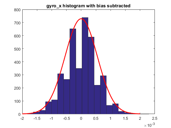
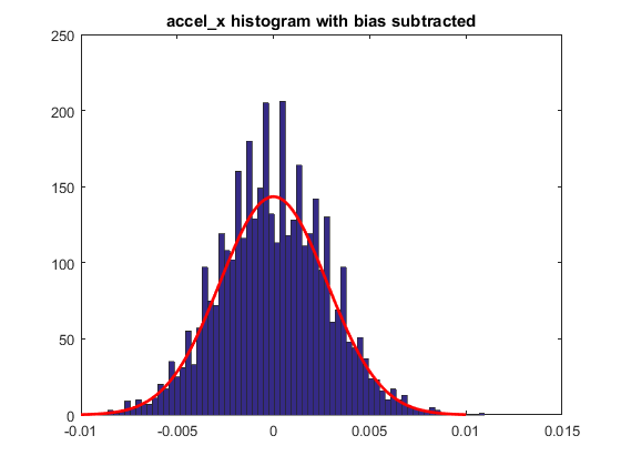
The sigma values for the three axes of the MPU6050 gyro and accels are shown below
| x | y | z | |
| Gyro | 5.4732e-04 | 6.1791e-04 | 6.2090e-04 |
| Accel | 2.8e-03 | 2.5e-03 | 3.8e-03 |
From this data, the measurement covariance matrix can be initialized directly as

Where the  denotes the std. dev of the standard deviation of the measurements along the x axis of the accelerometer as shown in the table above. For the process noise covariance, I set the part corresponding to the orientation as:

Multiplying with  models the uncertainty injected in each iteration of the Kalman filter and works well in practice, as we’ll see shortly. The part corresponding to the gyro bias can be set to some very low value as the gyro bias changes very slowly.
Sensor Simulator
In my experience working with real sensors and Kalman filtering, it takes a lot of trial and error to get your algorithms working. If you try to work with real data directly, bugs are very hard to debug since there are so many things that can go wrong. Therefore, it is important to come up with a simulation system that models the sensors using the chosen sensor parameters and generates simulated measurements that can be used as input to the sensor fusion algorithms.
To initialize the simulator, I create a “rotation trajectory” consisting of a series of orientation waypoints.
|
1 |
sim_state.trajectory_rotation = 1*[0 0 0; 20 20 20; 20 0 0; 20 20 0; 30 30 30; 0 0 0]*DEG2RAD; |
I then create a rotation path by interpolating between one waypoint to the next. This simple scheme will create sharp changes when transition from one waypoint to another occurs. A more sophisticated system will try to do some variant of spline fitting to create a smoother trajectory without abrupt changes. Here’s a good reference that describes the problem and discusses various solutions: smooth_trajectory .
|
1 2 3 4 5 6 7 8 9 10 11 12 13 14 15 16 17 18 19 20 |
for i = 1: num_wp-1 % beginning quaternion qa = eul2quat(sim_state.trajectory_rotation(i,1), sim_state.trajectory_rotation(i,2), sim_state.trajectory_rotation(i,3)); % ending quaternion qb = eul2quat(sim_state.trajectory_rotation(i+1,1), sim_state.trajectory_rotation(i+1,2), sim_state.trajectory_rotation(i+1,3)); ab = sim_state.trajectory_accel(i,:); % sim_state.accel beginning ae = sim_state.trajectory_accel(i+1,:); % sim_state.accel end % number of points on each segment of the trajectory num_points_segment = sim_state.num_sim_samples/num_segments; for j = 1: num_points_segment sim_state.orientation(idx,:) = interpolate_quat(qa, qb, j/num_points_segment); ap = ap + (ae-ab)/num_points_segment; sim_state.accel(idx,:) = ap + g'; sim_state.velocity(idx,:) = sim_state.velocity(idx-1,:)+(a_prev+ap)/2*time_step; sim_state.position(idx,:) = sim_state.position(idx-1,:) + (sim_state.velocity(idx,:)+sim_state.velocity(idx-1,:))/2*time_step; a_prev = ap; idx = idx + 1; end end end |
This code also attempts to create a trajectory for the position and velocity, but that can be ignored for now since those quantities are not part of our state vector. They will be later when we add image based measurements.
To generate measurement data, angular velocity necessary to transition from one orientation to the other is calculated and random noise and bias errors are added.
|
1 2 3 4 5 6 7 8 9 10 11 12 13 14 15 16 17 18 19 20 |
function [omega_measured, accel_measured, q_prev, dcm_true, q] = sim_imu_tick(sim_state, time_step, idx, sensor_model, q_prev) if (idx < sim_state.num_sim_samples) q = sim_state.orientation(idx,:); dcm_true = quat2dc(q); % dcm rotates from IMU to Global frame, dcm' does the opposite dq = (q - q_prev); q_prev = q; q_conj = [q(1) -q(2) -q(3) -q(4)]; % calculate the angular velocity required to go from one orientation to the next omega = 2*quatmult(q_conj, dq)/time_step; % take the vector part omega = omega(2:4); % add noise gyro_bias_noisy = sensor_model.gyro_bias + normrnd(0, sensor_model.gyro_bias_noise_sigma); omega_measured = omega' + normrnd(0, sensor_model.gyro_random_noise_sigma)+ gyro_bias_noisy; accel_measured = dcm_true'*sim_state.accel(idx,:)' + sensor_model.accel_bias + normrnd(0, sensor_model.accel_noise_sigma); % gyro_measurements(end+1,:) = omega_measured'; % accel_measurements(end+1,:) = accel_measured'; end end |
The sensor model is initialized from the statistics collected from the MPU6050 data logs, as explained above
|
1 2 3 4 5 6 7 8 9 10 11 12 13 14 15 16 17 18 19 20 21 22 23 24 25 26 27 28 29 30 31 32 33 34 35 36 37 38 39 40 41 42 43 |
function sensor_model = init_sensor_model(sensor_model, time_step) sensor_model.accel_noise_sigma = [0.003 0.003 0.004]'; % representative values for MPU6050 sensor_model.accel_noise_cov = (sensor_model.accel_noise_sigma).^2; sensor_model.accel_bias = [-0.06 0 0]'; % actual MPU6050 bias sensor_model.accel_bias_noise_sigma = [0.001 0.001 0.001]; sensor_model.R_accel = diag(sensor_model.accel_noise_cov); sensor_model.Q_accel_bias = diag(sensor_model.accel_bias_noise_sigma.^2); sensor_model.P_accel_bias = 0.1*eye(3,3); sensor_model.gyro_random_noise_sigma = [5.4732e-04 6.1791e-04 6.2090e-04]'; %rad/sec, representative values for MPU6050 sensor_model.gyro_bias_noise_sigma = 0.00001*ones(3,1); %rad/sec/sec. Any small value appears to work sensor_model.gyro_bias = [0.0127 -0.0177 -0.0067]'; % rad/sec sensor_model.Q_gyro_bias = diag(sensor_model.gyro_bias_noise_sigma.^2); % position uncertainity sensor_model.Q_p = diag(sensor_model.accel_noise_cov)*time_step; % velocity uncertainity sensor_model.Q_v = diag(sensor_model.accel_noise_cov)*time_step; % quaternion (orientation) uncertainity sensor_model.Q_q = diag(sensor_model.gyro_random_noise_sigma.^2)*time_step; % Initial values for various elements of the covariance matrix. Only % effects the transient behaviour of the filter, not the steady state % behaviour. sensor_model.P_p = 0.1*eye(3,3); sensor_model.P_v = 0.1*eye(3,3); sensor_model.P_q = 0.1*eye(3,3); sensor_model.P_gyro_bias = 0.1*eye(3,3); sensor_model.P_accel_bias = 0.1*eye(3,3); end |
Let’s now look at the calculations during each iteration of the filter.
|
1 2 3 4 5 6 7 8 9 10 11 12 13 14 15 16 17 18 19 20 21 22 23 24 25 26 27 28 29 30 31 32 33 34 35 36 37 38 39 40 41 42 43 44 45 46 47 48 49 50 51 52 53 54 55 56 57 58 59 60 61 62 63 64 65 66 67 68 69 70 71 72 73 74 75 76 77 |
for i = 2:num_sim_samples idx = i; % Get current sensor values from the simulator [omega_measured, accel_measured, q_prev, dcm_true, q_true] = sim_imu_tick(sim_state, time_step, idx, sensor_model, q_prev); % Calculate estimated values of omega and accel by subtracting the % estimated values of the biases omega_est = omega_measured - sv.gyro_bias_est; accel_est = accel_measured - sv.accel_bias_est; phi = omega_est*time_step; delta_vel = accel_est*time_step; % not necessary for accel-gyro sensor fusion phi3 = make_skew_symmetric_3(phi); % update current orientation estimate. We maintain orientation estimate % as a quaternion and obtain the corresponding DCM whenever needed sv.q_est = apply_small_rotation(phi, sv.q_est); sv.dcm_est = quat2dc(sv.q_est); % Integrate accel (after transforming to global frame) to obtain % velocity and position orig_velocity = sv.velocity_est; sv.velocity_est = sv.velocity_est + sv.dcm_est*delta_vel - g*time_step ; final_velocity = sv.velocity_est; sv.position_est = sv.position_est + ((orig_velocity + final_velocity)/2)*time_step; % State transition matrix F = eye(6) + [-phi3 eye(3)*time_step; zeros(3,6)]; % propagate covariance P = F*P*F' + Qd; % Apply accelerometer measurements. if (mod(i, accelUpdateFrequency) == 0) % apply accel measurements. The updated state vector and covariance % matrix are returned. [sv, P] = process_accel_measurement_update2(sv, accel_est, P, sensor_model.R_accel, g); gyro_bias_est = sv.gyro_bias_est; q_est = sv.q_est; dcm_est = sv.dcm_est; end end function q_est = apply_small_rotation(phi, q_est) s = norm(phi)/2; x = 2*s; phi4 = make_skew_symmetric_4(phi); % approximation for sin(s)/s sin_sbys_approx = 1-s^2/factorial(3) + s^4/factorial(5) - s^6/factorial(7); exp_phi4 = eye(4)*cos(s) + 1/2*phi4*sin_sbys_approx; % method 1 q_est1 = exp_phi4*q_est; % verify: should be equal to: % method 2 (direct matrix exponential) q_est2 = expm(0.5*(phi4))*q_est; % verify should be equal to: % method 3: propagate by quaternion multiplication (doesn't preserve unit % norm) dq = [1 phi(1)/2 phi(2)/2 phi(3)/2]; dq_conj = [1 -phi(1)/2 -phi(2)/2 -phi(3)/2]'; q_est3 = quatmul(q_est, dq'); q_est = q_est1; end function phi4 = make_skew_symmetric_4(phi) phi4 = [0 -phi(1) -phi(2) -phi(3); phi(1) 0 phi(3) -phi(2); phi(2) -phi(3) 0 phi(1); phi(3) phi(2) -phi(1) 0]; end |
Let’s see what happens if we run this code without applying any accelerometer updates (we’ll discuss those in a second). We start with zero for our estimated value of the gyro biases. Due to the bias and random noise in the gyro measurments, we expect the estimated orientation to gradually drift from the true orientation and the covariance of the error state to grow with every iteration. As the two videos below show, this is indeed what happens.
Let’s now add the accelerometer updates. The relevant code is shown below. The code implements the math we developed earlier.
|
1 2 3 4 5 6 7 8 9 10 11 12 13 14 15 16 17 18 19 20 21 22 23 24 25 26 27 28 29 30 31 32 33 34 35 36 37 38 39 40 41 42 43 44 45 46 47 48 49 50 51 52 53 54 |
% reduced model, applies to accel+gyro only. No camera function [state, P] = process_accel_measurement_update2(state, accel_est, P, R_accel, g) % current estimated states q_est = state.q_est; dcm_est = state.dcm_est; gyro_bias_est = state.gyro_bias_est; % Calculate residual (in the global reference frame) accel_residual = dcm_est*accel_est - g; % Construct the H matrix H_accel = [-make_skew_symmetric_3(g)*dcm_est zeros(3,3)]; % Calculate Kalman Gain K_gain = P*H_accel'*inv([H_accel*P*H_accel' + R_accel]); % Calculate the correction to the error state x_corr = K_gain*accel_residual; % Calculate the new covariance matrix P = P - K_gain*H_accel*P; % Apply the updates to get the new state x_est = apply_accel_update(x_corr, [q_est; gyro_bias_est]); gyro_bias_est(1:3) = x_est(5:7); q_est = x_est(1:4); %ness = [x_corr(1:2) x_corr(4:5)]'*inv(P(1:2, 1:2))*x_corr(1:2); ness = x_corr'*inv(P)*x_corr; % Update state vector state.q_est = q_est; state.dcm_est = dcm_est; state.gyro_bias_est = gyro_bias_est; end function x_est = apply_accel_update(x_corr, x_est) % gyro bias x_est(5:7) = x_est(5:7) + x_corr(4:6); % orientation update phi = -[x_corr(1) x_corr(2) x_corr(3)]; phi3 = make_skew_symmetric_3(phi); phi4 = make_skew_symmetric_4(phi); s = norm(phi)/2; sin_sbys_approx = 1-s^2/factorial(3) + s^4/factorial(5) - s^6/factorial(7); exp_phi4 = eye(4)*cos(s) + 1/2*phi4*sin_sbys_approx; x_est(1:4) = exp_phi4*x_est(1:4); end |
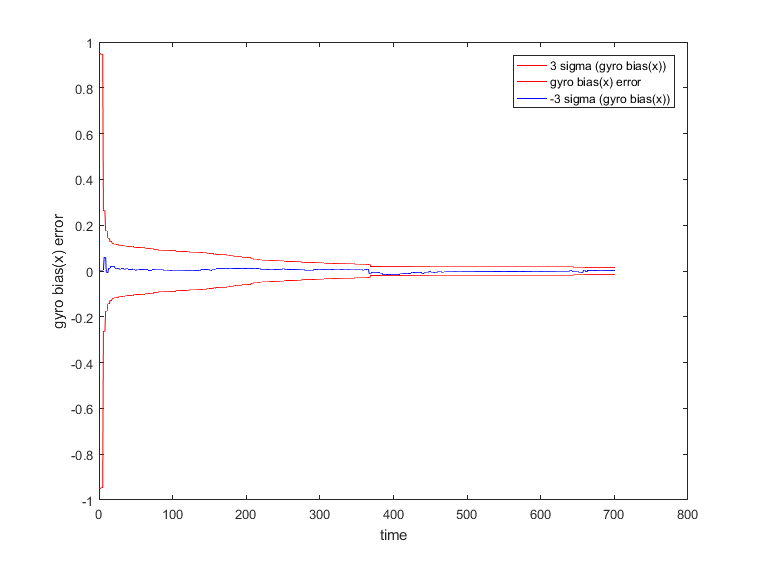
Adding the accelerometer update correctly estimates the gyro bias and corrects for the drift in pitch and roll. The final estimated gyro bias is shown below.
| x | y | z | |
| Estimated Gyro bias | 0.0127 | -0.0179 | -0.0069 |
As mentioned in 2, a good way to visualize if the Kalman filter is performing well is to compare the range of variation of the residuals (difference between the true and estimated states) with the corresponding element of the covariance matrix. When the filter is performing optimally, the residuals should lie within the corresponding sigma bound. For example, approximately 99% of the residuals should lie between  . We show the variation of the error along the x-axis (roll error) and plot it along the
  .
.  is obtained by taking the square root of the first element of the covariance matrix.
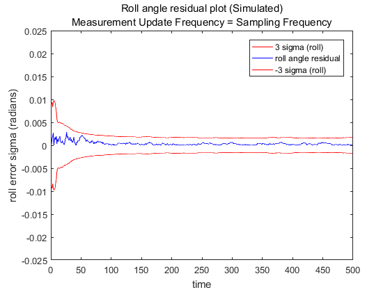
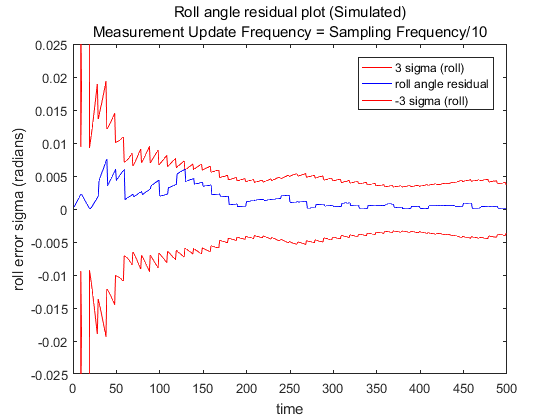
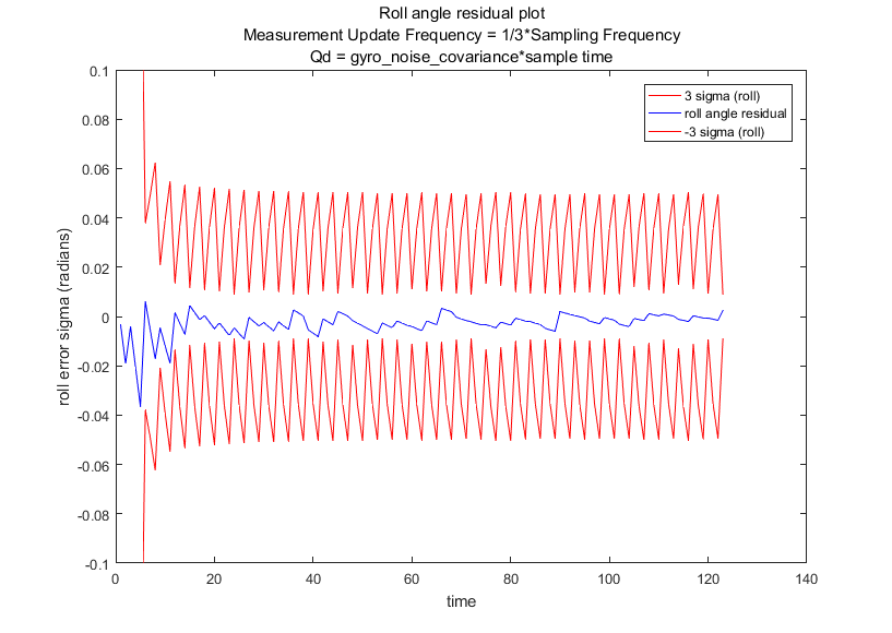
Here, the accelerometer measurement updates are being applied every step of the iteration. If we apply the updates less frequently, we can see the jaggedness in the graph for . The jaggedness occurs because the covariance increases between successive measurement updates and is brought down when the update is applied. The covariance converges in both cases, however as one might expect, it converges to a higher value when the accelerometer updates are applied less frequently.

From equation 1, it can be seen that when the axis of rotation aligns with the current orientation,  , where is a scalar. Hence
  . Therefore rotation along the current orientation (local vertical) doesn’t change the accelerometer residual, and is therefore unobservable.
A few more observations. The choice of the initial value of the covariance matrix only affects the transient behaviour of the filter and doesn’t change the final (converged) value of the covariance. Therefore, this matrix can be set to a diagonal matrix with suitably low values. The process noise covariance matrix does affect the final covariance matrix and can be used as a design parameter to weigh the gyro and accel measurements suitably. We set this matrix to a diagonal matrix with the terms corresponding to the orientation errors equal to the square of the standard deviation of the gyro measurements multiplied by the time step. The intuition being that this reflects the uncertainty injected in every update step. The terms corresponding to the gyro bias error can be set to a very low value as the bias changes very slowly.
To evaluate the performance of this filter implementation on real data, I applied the kalman filtering to IMU data being streamed in over a serial port. The data was collected by connecting the MPU6050 to an Arduino over a I2C connection and the raw data was sent to the PC over a serial port connection. Matlab provides APIs for receiving data over a serial port by setting up a function callback which made it easy to switch the data source to be live data instead of simulated data (contact me for the code). The sensor fusion results for live data are similar to that obtained for simulated data, except for one difference. As noted above, accelerometer measurements don’t provide observability for orientation changes along the axis of rotation and thus I disabled the update for the gyro bias error along the local z-axis. Enabling this update would cause the gyro bias along the local z-axis to become unstable and thereby lead to errors in orientation.
The plot of orientation and gyro bias errors and the corresponding  are shown below. In general, we don’t know the true orientation for live data without expensive calibration steps. In my case, I kept the IMU on a flat surface and measured the orientation along one of the axes by calculating the angle from accelerometer data.
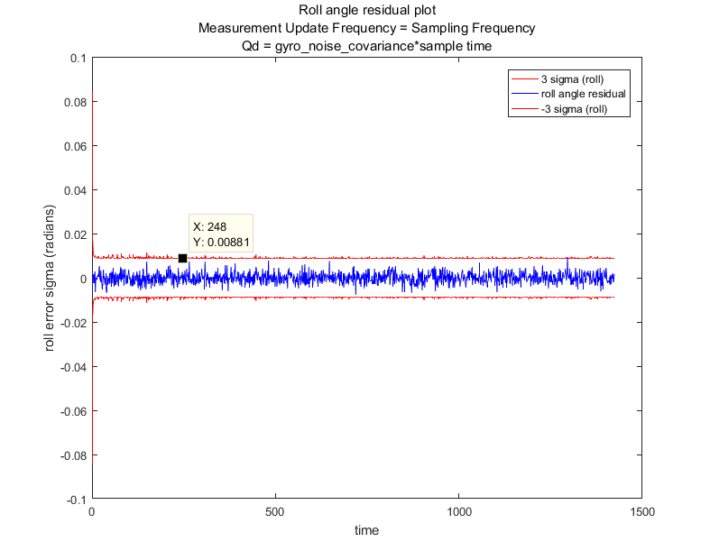
In the next post, we’ll expand our state vector to include position and velocity and add image measurements.
Hi! thank you for your work! This is very helpful to me!
Can I ask some?
1. Can I get an IMU data we used?
2. Did you try to add Magnetometer data?
Thank you very much!
First of all, thank you very much for your work!
This is very helpful to me!!
Can you do me a favor?
1. Can I get a raw data of this?
2. Did you try to fuse Magnetometer data for yaw angle?
Thank you
Sorry, I don’t have the raw data anymore. I didn’t use magnetometer for yaw correction, which is a common technique to do yaw correction. I do show the math for the magnetometer measurement update.
Thank you very much for sharing the knowledge and this great post.
Could you please open source the code for Sensor Fusion part 3 and part 4.
I’ve posted the code on github and added a link (in part 4).
Great Post. It is very helpful.