

In this post, we’ll add the math and provide implementation for adding image based measurements. Let’s recap the notation and geometry first introduced in part 1 of this series
The state vector in equation 16 of 1 consists of 21 elements.
 : Error in the position of the IMU in the global reference frame
 : Error in the velocity of the IMU in the global reference frame
 : Error in the orientation between the IMU and the global reference frame
 : Error in the position of the camera with respect to the IMU
 : Error in the orientation between the camera and the IMU
 : Error in gyro bias
 : Error in accel bias
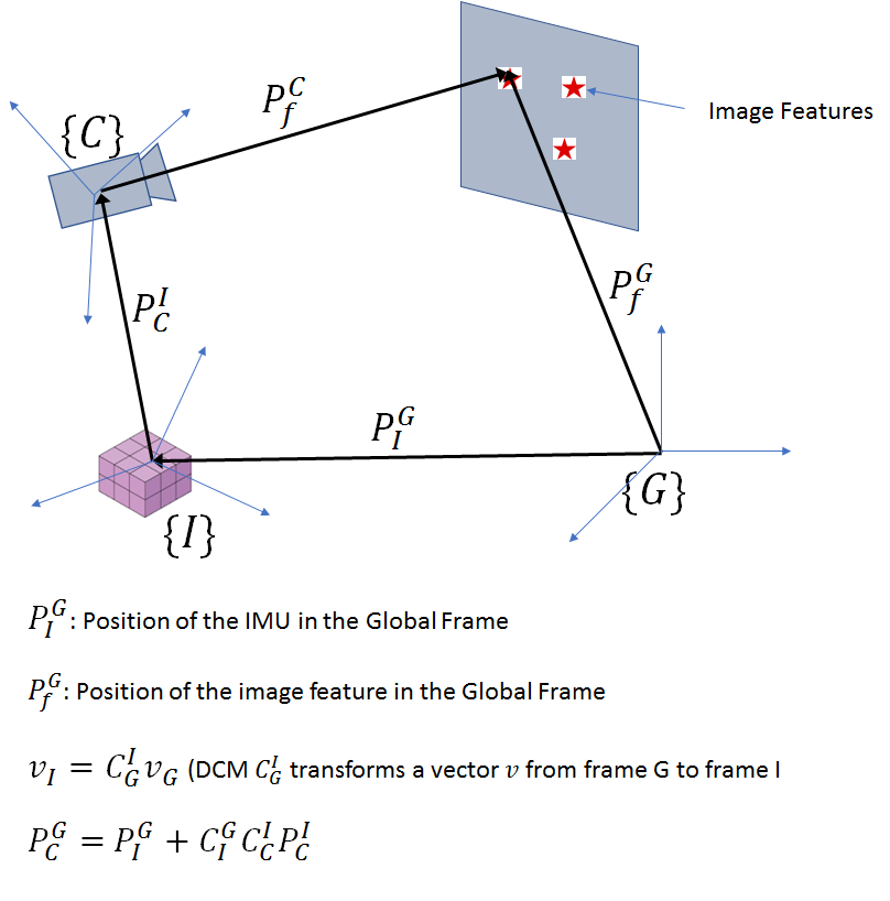
This is a 21 element state vector with the camera-IMU offset as one of its elements. We’ll consider a simpler problem first where the IMU is aligned with the camera. Thus, our state vector consists of the errors in the position, velocity and orientation of the IMU (or Camera) wrt the global frame and the gyro and accel bias errors. The imaged feature points provide measurements that will be used to correct our estimates of position, velocity, orientation, gyro and accel bias.
In the previous posts, we already derived the state propagation equations for gyro bias and orientation errors. Let’s now derive the propagation equations for the accel bias, position and velocity. As before, for a variable  ,
,  denotes the measured quantity,
  denotes the estimated quantity and
  denotes the error. From the laws of motion,

and therefore,
(1) 
I’m not using bold for  as it is obvious from the notation that these are vector quantities.

Taking the derivative,


Note that since there are now multiple DCMs, I’m explicitly stating the coordinate systems a given DCM acts on. For example,  transforms a vector from the global to the IMU-Camera coordinate system. Also, I’m using a prime to denote transpose, so
  .
.
From post 2 of this series,
![\delta{\dot{V_{I}^{G}}} = \hat{C}^{'G}_{I}(\boldsymbol{a_m} - \boldsymbol{\hat{a_b}}) - (\hat{C}^{'G}_{I} + \hat{C}^{'G}_{I}[\delta\theta]^{'}_{\times})\boldsymbol{a}](https://www.telesens.co/wp-content/ql-cache/quicklatex.com-795382a0eb027354f7e45a2c02d7bad9_l3.png "Rendered by QuickLaTeX.com")
Now, since  ,
,  and
and ![[\delta\theta]^{'}_{\times} = -[\delta\theta]_{\times}](https://www.telesens.co/wp-content/ql-cache/quicklatex.com-38a9b67efee0591ce26677bc17f0e31b_l3.png "Rendered by QuickLaTeX.com") ,
,
![\delta{\dot{V_{I}^{G}}} = -\hat{C}^{'G}_{I}(\delta{\boldsymbol{a_b}}) + \hat{C}^{'G}_{I}[\delta\theta]_{\times}\boldsymbol{a}](https://www.telesens.co/wp-content/ql-cache/quicklatex.com-570767ac965a103bdf133ca66da587aa_l3.png "Rendered by QuickLaTeX.com")
From the first post, we know that ![[a]_{\times}\boldsymbol{b} = -[b]_{\times}\boldsymbol{a}](https://www.telesens.co/wp-content/ql-cache/quicklatex.com-7abc3e74f9e78e9ff05901fb0117d51b_l3.png "Rendered by QuickLaTeX.com") . Thus,
. Thus,
(2) ![\begin{equation*}\delta{\dot{V_{I}^{G}} = -\hat{C}^{'G}_{I}\delta{\boldsymbol{a_b}} - \hat{C}^{'G}_{I}[a]_{\times}\boldsymbol{\delta\theta}\end{equation*}](https://www.telesens.co/wp-content/ql-cache/quicklatex.com-b342f5e3a59e9ad35f4a7053ce5fd74e_l3.png "Rendered by QuickLaTeX.com")
Similar to the gyro bias, the accel bias changes very slowly and therefore the error in the accel bias can be assumed to be constant over the time step.
(3) 
Combining the equations 1,2,3 with the state propagation equations for the orientation and gyro bias errors developed in the previous posts, the entire  state transition matrix is given as:
(4) ![\begin{equation*}\begin{bmatrix}\dot{\delta{P_{I}^{G}}} \\ \dot{\delta{V_{I}^{G}}} \\ \dot{\delta{\boldsymbol{\theta}}} \\ \dot{\delta{\boldsymbol{g_b}}} \\ \dot{\delta{\boldsymbol{a_b}}}\end{bmatrix} = \begin{bmatrix} 0_{3\times3} & I_{3\times3} & 0_{3\times3} & 0_{3\times3} & 0_{3\times3} \\ 0_{3\times3} & 0_{3\times3} & - \hat{C}^{'G}_{I}[a]_{\times} & 0_{3\times3} & -\hat{C}^{'G}_{I} \\ 0_{3\times3} & 0_{3\times3} & [\phi]_{\times} & I_{3\times3} & 0_{3\times3} \\ 0_{3\times3} & 0_{3\times3} & 0_{3\times3} & 0_{3\times3} & 0_{3\times3} \\ 0_{3\times3} & 0_{3\times3} & 0_{3\times3} & 0_{3\times3} & 0_{3\times3}\end{bmatrix}\begin{bmatrix}\delta{P_{I}^{G}} \\ \delta{V_{I}^{G}}\\ \delta{\boldsymbol{\theta}} \\ \delta{\boldsymbol{g_b}} \\ \delta{\boldsymbol{a_b}}\end{bmatrix}\end{equation*}](https://www.telesens.co/wp-content/ql-cache/quicklatex.com-4de7337ad33028ebd2ba2c56c7c9fda3_l3.png "Rendered by QuickLaTeX.com")
Thus,
(5) ![\begin{equation*}J = \begin{bmatrix} 0_{3\times3} & I_{3\times3} & 0_{3\times3} & 0_{3\times3} & 0_{3\times3} \\ 0_{3\times3} & 0_{3\times3} & - \hat{C}^{'G}_{I}[a]_{\times} & 0_{3\times3} & -\hat{C}^{'G}_{I} \\ 0_{3\times3} & 0_{3\times3} & [\phi]_{\times} & I_{3\times3} & 0_{3\times3} \\ 0_{3\times3} & 0_{3\times3} & 0_{3\times3} & 0_{3\times3} & 0_{3\times3} \\ 0_{3\times3} & 0_{3\times3} & 0_{3\times3} & 0_{3\times3} & 0_{3\times3}\end{bmatrix}\end{equation*}](https://www.telesens.co/wp-content/ql-cache/quicklatex.com-bbb6cdae9b745147f71ff79109a13e2b_l3.png "Rendered by QuickLaTeX.com")
As before, the state transition matrix  is given by:
(6) 
The covariance is propagated as:
(7) 
Here  is the time step index.
Let’s now look at the measurement update equations. The simplified geometry given that the IMU and the camera are coincident is shown below:
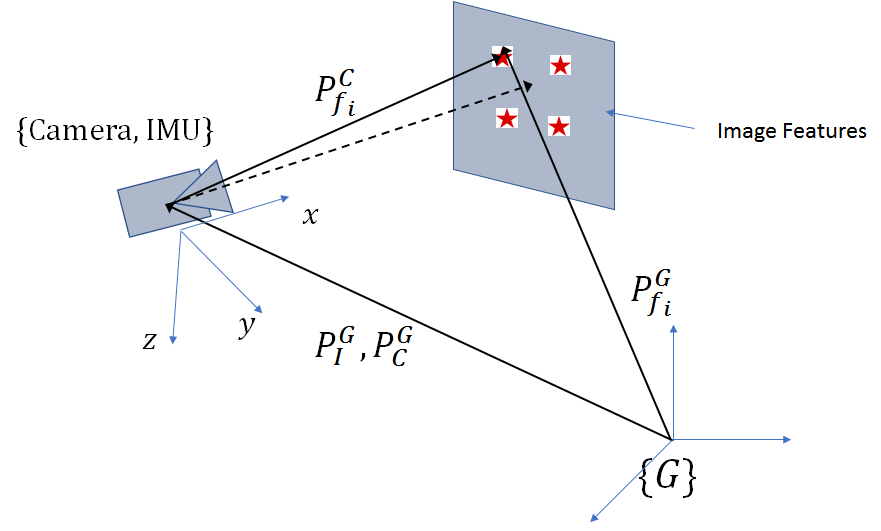
Note that in our coordinate system, the axis is oriented along the optical axis of the camera and the  axis points down. This follows the convention used on the MPU6050 IMU. In computer vision, it is more common for the axis to be pointed along the optical axis.
Let the 3D position of the feature point  be represented by
  in the global coordinate system. Denoting the camera calibration matrix by
  , the projection of this point,
  is given by:

Here is a  matrix:

Here  denotes the focal length and
  and
and  the image center. We assume a rectilinear camera with square pixels with no radial and tangential distortion. Those terms can be added easily if needed.
The final image coordinates are obtained by applying the perspective divide.

The jacobian matrix consists of the partial derivatives of the image coordinates against the parameters we are trying to estimate, i.e., and  . To obtain the expressions for the partial derivatives, it is useful to think of the perspective projection and coordinate transformation as a function composition and then apply the chain rule. From the chain rule,

Here  is the coordinate transformation function that maps the vector
  from the global coordinate system to vector
  in the camera-IMU coordinate system.
  then applies the perspective divide on the vector .
From straightforward differentiation,

Let’s denote the matrix represented by  by
by  .
.
Now let’s consider 

From the vector calculus results derived in part 1,
![g^{'}(\boldsymbol{x}) = \begin{bmatrix}KC_G^I[P_{f_i}^G - P_I^G]_{\times}\boldsymbol{\delta\theta} & -KC_G^I\delta{P_{I}^{G}}\end{bmatrix}](https://www.telesens.co/wp-content/ql-cache/quicklatex.com-a304460dda82438be6871d9dedb32035_l3.png "Rendered by QuickLaTeX.com")
The derivatives against the other elements of the state vector are 0. Therefore (after replacing  and
and  by their estimated versions), the measurement update matrix
  is given as:
(8) ![\begin{equation*} H_{image} = M\begin{bmatrix}-K\hat{C}_G^I & 0_{3\times3} & K\hat{C}_G^I[P_{f_i}^G - \hat{P}_I^G]_{\times} & 0_{3\times3} & 0_{3\times3} \end{bmatrix}\end{equation*}](https://www.telesens.co/wp-content/ql-cache/quicklatex.com-b9331b99253465e66619ddb6e35fe7b6_l3.png "Rendered by QuickLaTeX.com")
Simulation Setup
Our simulation set up consists of a camera and IMU located coincident to each other. In the initial position, the optical axis of the camera is pointed along positive . The camera is looking at four feature points located a few units away symmetrically around the optical axis. The position of these feature points in the world (global) coordinate system is assumed to be known. During the simulation, the camera + IMU translates and rotates along a predefined trajectory. From this trajectory, simulated sensor measurements are generated by calculating the incremental angular velocities and accelerations and adding bias and noise according to our sensor model. Simulated image measurements are also generated by applying coordinate transformation and perspective projection to the feature points and adding gaussian pixel noise.
State estimation is performed by integrating noisy angular velocities and accelerations (after adjusting for estimated gyro and accel bias) to obtain estimated orientation, position and velocity. The state covariance matrix is propagated according to eq (7). The noise image measurements are then used as a measurement source to correct for the errors in the state vector.
It is well known that integrating noisy accelerometer data to estimate velocity and double integrating to obtain position leads to quick accumulation of errors. The error in the position and orientation will cause the estimated image measurements to drift away from the true measurements (the difference between the two acts as a source of measurement). The video below shows this drift. The camera in the video was held stationary and thus the image projection of the feature points should not move (except for the small perturbation caused by pixel noise).
Let’s also take a look at our simulated trajectory. We use a cube as prop to show the movement of the camera +IMU along the simulated trajectory.
Now let’s look at some of the Matlab code that implements one iteration of the Kalman filter operation.
|
1 2 3 4 5 6 7 8 9 10 11 12 13 14 15 16 17 18 19 20 21 22 23 24 25 26 27 28 29 30 31 32 33 34 35 36 37 38 39 40 41 42 43 44 45 |
% Obtain simulated IMU measurements [omega_measured, accel_measured, q_prev] = sim_imu_tick(sim_state, time_step, idx, sensor_model, q_prev); % Obtain simulated camera measurements. p_f_in_G contains the feature % locations and p_C_in_G the camera location in the global coordinate system % sigma_image is the std. dev of the pixel noise, K the camera % calibration matrix. image_measurements = sim_camera_tick(dcm_true, p_f_in_G, p_C_in_G, K, numFeatures, sigma_image); % Obtain estimated values by adjusting for current estimate of the % biases omega_est = omega_measured - sv.gyro_bias_est; accel_est = accel_measured - sv.accel_bias_est; % Multiply by time_delta to get change in orientation/position phi = omega_est*time_step; vel = accel_est*time_step; vel3 = make_skew_symmetric_3(vel); phi3 = make_skew_symmetric_3(phi); % Generate new estimates for q, position, velocity using equations of motion sv = update_state(sv, time_step, g, phi, vel); % State transition matrix F = eye(15) + [zeros(3,3) eye(3)*time_step zeros(3,3) zeros(3,3) zeros(3,3); zeros(3,3) zeros(3,3) sv.dcm_est*vel3 zeros(3,3) -sv.dcm_est*time_step; zeros(3,3) zeros(3,3) -phi3 eye(3)*time_step zeros(3,3); zeros(3,15); zeros(3,15)]; % Propagate covariance P = F*P*F' + Qd; % Apply image measurement update if (mod(i, image_update_frequency) == 0) [sv, P] = process_image_measurement_update(sv, p_f_in_G, image_measurements, ... numFeatures, P, K, imageW, imageH, sigma_image); end function image_measurements = sim_camera_tick(dcm_true, p_f_in_G, p_C_in_G, K, numFeatures, sigma_image) for fid = 1: numFeatures % feature position in camera frame fic = dcm_true'*(p_f_in_G(fid,:) - p_C_in_G')'; % apply perspective projection and add noise image_measurements(2*fid-1:2*fid) = K*[fic(2)/fic(1) fic(3)/fic(1) 1]' ... + normrnd(0, [sigma_image sigma_image]'); end end |
Let’s first see what happens if no image updates are applied.
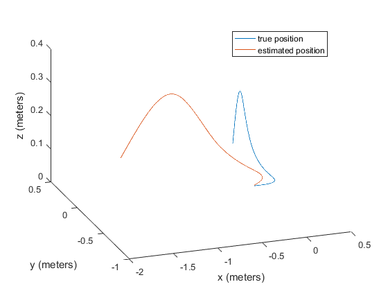
We can see that the estimated position very quickly diverges from the true position. Let’s now look at the code for the image measurement update.
|
1 2 3 4 5 6 7 8 9 10 11 12 13 14 15 16 17 18 19 20 21 22 23 24 25 26 27 28 29 30 31 32 33 34 35 36 37 38 39 40 41 42 43 44 45 46 47 48 49 50 51 52 |
% Iterate until the CF < 0.25 or max number of iterations is reached while(CF > 0.25 && numIter < 10) numIter = numIter + 1; estimated_visible = []; measurements_visible = []; residual = []; for indx = 1:numVisible % index of this feature point fid = visible(indx); % estimated position in the camera coordinate system fi_e = dcm_est'*(p_f_in_G(fid,:)' - p_C_in_G_est); % feature in image, estimated % focal lengths (recall that the x axis of our coordinate % system points along the optical axis) fy = K(1,1); fz = K(2,2); J = [-fy*fi_e(2)/fi_e(1).^2 fy*1/fi_e(1) 0; -fz*fi_e(3)/fi_e(1).^2 0 fz*1/fi_e(1)]; % Measurement matrix H_image(2*indx-1: 2*indx,:) = [-J*dcm_est' zeros(2,3) ... J*dcm_est'*make_skew_symmetric_3((p_f_in_G(fid,:)' - p_C_in_G_est)) zeros(2,3) zeros(2,3)]; % estimated image measurement estimated_visible(2*indx-1: 2*indx) = K*[fi_e(2)/fi_e(1) fi_e(3)/fi_e(1) 1]'; % actual measurement measurements_visible(2*indx-1: 2*indx) = measurements(2*fid-1: 2*fid)'; end % vector of residuals residual = estimated_visible - measurements_visible; %show_image_residuals(f4, measurements_visible, estimated_visible); % Kalman gain K_gain = P*H_image'*inv([H_image*P*H_image' + R_im]); % Correction vector x_corr = K_gain*residual'; % Updated covariance P = P - K_gain*H_image*P; % Apply image update and correct the current estimates of position, % velocity, orientation, gyro/accel bias x_est = apply_image_update(KF_SV_Offset, x_corr, ... [position_est; velocity_est; q_est; gyro_bias_est; accel_bias_est]); position_est = x_est(KF_SV_Offset.pos_index:KF_SV_Offset.pos_index+KF_SV_Offset.pos_length-1); velocity_est = x_est(KF_SV_Offset.vel_index:KF_SV_Offset.vel_index+KF_SV_Offset.vel_length-1); gyro_bias_est = x_est(KF_SV_Offset.gyro_bias_index:KF_SV_Offset.gyro_bias_index + KF_SV_Offset.gyro_bias_length-1); accel_bias_est = x_est(KF_SV_Offset.accel_bias_index:KF_SV_Offset.accel_bias_index + KF_SV_Offset.accel_bias_length-1); q_est = x_est(KF_SV_Offset.orientation_index:KF_SV_Offset.orientation_index+KF_SV_Offset.orientation_length-1); dcm_est = quat2dc(q_est); p_C_in_G_est = position_est; % Cost function used to end the iteration CF = x_corr'*inv(P)*x_corr + residual*R_inv*residual'; end |
The code follows the equation for the image measurement update developed earlier. One difference between image measurement update and accelerometer update discussed in the last post is that we run the image measurement update in a loop until the cost function defined in equation (24) of 1 is lower than a threshold or the maximum number of iterations is reached.
Let’s look at the trajectory with the image updates applied at 1/10 the IMU sampling frequency with two values of image noise sigma
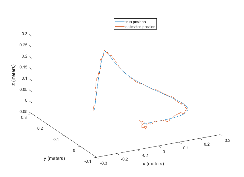
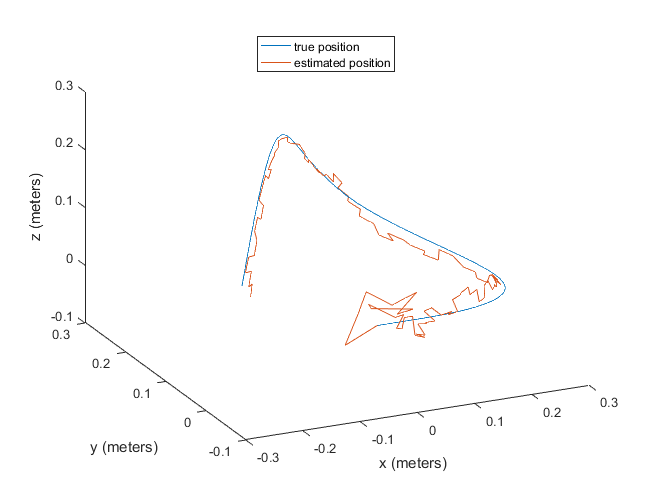
As we can see, adding the image measurement update prevents any systematic error in position from developing and keeps the estimated position wandering around the true position. The amount of wander is higher for higher value of image noise sigma, as expected. The wander around the starting point is likely due to the kalman filter in the process of estimating the gyro and accel biases and converging to a steady state. Once the biases have been estimated and the covariance has converged, the estimated position tracks the true position closely.
The system also correctly estimates the accel and gyro biases. The true and estimated biases for the two different values of image noise sigma are shown below.
| Gyro (x) | Gyro (y) | Gyro (z) | Accel (x) | Accel (y) | Accel (z) | |
| True | 0.0127 | -0.0177 | -0.0067 | -0.06 | 0 | 0 |
Estimated ( = 0.1) = 0.1) |
0.0126 | -0.0176 | -0.0067 | -0.0581 | 0.0053 | 0.0010 |
| Estimated ( = 0.5) |
0.0127 | -0.0175 | -0.0071 | -0.0736 | 0.0031 | -0.0092 |
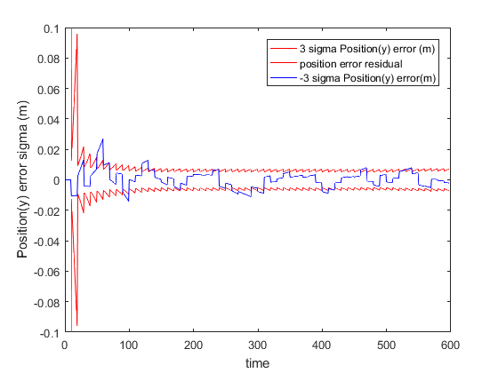
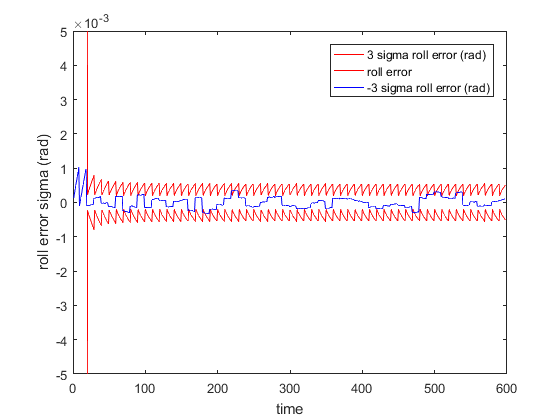
The residual plots for the position (along y axis) and orientation (roll) are shown below. The residuals mostly lie between the corresponding 3 sigma bounds and thus the filter appears to be performing well.
As suggested in 2, it is better to maintain the covariance matrix in UD factorized form for better numerical stability and efficient calculation of matrix inverse. We have not implemented this optimization.
The full source code is available here.
Implementing a Real System
Our simulation results look quite promising, and thus it is time to implement a real, working system. A real system will present many challenges –
- Picking suitable feature points in the environment and computing their 3D positions is not easy. Some variant of epipolar geometry based scene geometry computation plus bundle adjustment will have to be implemented.
- Some way of obtaining the correspondence between 3D feature points and their image projections will have to be devised.
- Image processing is typically a much slower operation than processing IMU updates. It is quite likely that in a real system, updates from the image processing module are stale by the time they arrive and thus can’t be applied directly to update the current covariance matrix. This time delay will have to be factored in the implementation of the covariance update.
Leave a Reply