

In the previous post, I showed you how the cord19q ETL system parses documents in the Covid-19 corpus into a SQLite database. In this post, I’ll go over the rest of the ETL process and the query lookup process. The application source code is here. The rest of the ETL process consists of the following three steps:
- Creating high quality vector representations (word embeddings) of words in the entire corpus that group similar words closer together.
- Calculating BM25 statistics of important words in relevant sentences. BM25 is a ranking function used to reward relevance by assigning higher scores to more important words with higher information value. It is a variant of the popular TF-IDF ranking function.
- Using the output of steps 1 and 2 to calculate the embedding representation of relevant sentences which can be used to find sentences relevant to a given query. This embedding representation is the weighted average of the embeddings of the important words comprising a sentence, with the BM25 scores used as the weights.
Notice that steps 2 and 3 are carried out for relevant sentences only. There are 16339099 sentences in the entire corpus. Out of these, only sentences that are marked with the COVID-19 tag and are not fragments or questions and don’t come from sections such as Introduction or Background are considered relevant. This filtering process reduces the number of sentences to be considered during the similarity search to 917986 which reduces storage requirements and speeds up sentence similarity lookup at query time.
Similarly, the BM25 scores are only calculated for important words in a sentence. For example, stop words such as “and”, “but”, words with fewer than 2 characters etc., are excluded.
Let’s go over each of the three steps in more detail.
Table of Contents
Calculating word embeddings (also known as word vectors)
Word embeddings are a type of word representation that allows words with similar meaning to have a similar representation. Representing words by learnt embeddings is a fundamental advance in natural language understand and is usually a starting point for most natural language processing workflows. I’ll introduce the basic idea here and then refer you to some papers and articles for more information.
Consider the following similar sentences: Have a good day and Have a great day. We know from prior knowledge that these sentences have a similar meaning. If these are the only two sentences in our corpus, an exhaustive vocabulary (let’s call it V) would be V = {Have, a, good, great, day}.
How can be represent the words in this vocabulary? A trivial choice is to create a one-hot encoded vector for each of these words in V. Length of our one-hot encoded vector would be equal to the size of V (=5). These one-hot vectors would like this:
Have: ![[1, 0, 0, 0, 0]](https://www.telesens.co/wp-content/ql-cache/quicklatex.com-2a9eacf9d62a7d9d54a87180907a4c2c_l3.png "Rendered by QuickLaTeX.com") , a:
, a: ![[0, 1, 0, 0, 0]](https://www.telesens.co/wp-content/ql-cache/quicklatex.com-0484d7799195c1420c13b287aed15d26_l3.png "Rendered by QuickLaTeX.com") , good:
, good: ![[0, 0, 1, 0, 0]](https://www.telesens.co/wp-content/ql-cache/quicklatex.com-067795eb15848ff2dfb55493dd1dde2d_l3.png "Rendered by QuickLaTeX.com") , great:
, great: ![[0, 0, 0, 1, 0]](https://www.telesens.co/wp-content/ql-cache/quicklatex.com-135af567dbab230b401cb81d2faede6c_l3.png "Rendered by QuickLaTeX.com") , day:
, day: ![[0, 0, 0, 0, 1]](https://www.telesens.co/wp-content/ql-cache/quicklatex.com-3233d5e4190e587017c9b2ea5c3c4b54_l3.png "Rendered by QuickLaTeX.com") . These vectors are all mutually orthogonal, meaning that the angle between vectors corresponding to “good” and “great” is the same as between “good” and “have”. We know that this is not true; “good” and “great” and semantically closer to each other than “good” and “have”. Furthermore, using a one-hot encoding representation means that the size of a word vector is equal to the size of the vocabulary which for natural languages can be easily in the hundreds of thousands.
. These vectors are all mutually orthogonal, meaning that the angle between vectors corresponding to “good” and “great” is the same as between “good” and “have”. We know that this is not true; “good” and “great” and semantically closer to each other than “good” and “have”. Furthermore, using a one-hot encoding representation means that the size of a word vector is equal to the size of the vocabulary which for natural languages can be easily in the hundreds of thousands.
Learnt word embeddings aim to automatically learn word representations that are compact (usually 128 or 256 dimensions) and can capture the semantic relationship between words. It does so by using a fundamental linguistic assumption called the distributional hypothesis which states that words appearing in similar contexts are related to each other semantically. For more info, see the original word embedding paper and the Pytorch example that shows how word embeddings can be learnt in an unsupervised manner from a large corpus of text.
The family of techniques used to calculate word embeddings from a body of text are called “word2vec”. The cord19q ETL system uses a fast and memory efficient implementation of word2vec called FastText.
The flowchart used to create the word embeddings is shown below.
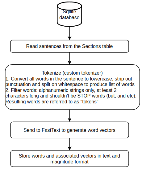
FastText takes two configuration parameters – embedding dimension (set to 300) and mincount (set to 3), which is the minimum number of times a token must appear for creating an embedding. The other parameters used in the word2vec algorithm such as the model type, learning rate, number of epochs, context window size etc., are left to their default values.
|
1 2 |
# Train on tokens file using largest dimension size model = fasttext.train_unsupervised(tokens, dim=size, minCount=mincount) |
Output files
The default cord19q ETL system saves word embeddings in two formats – plain text and magnitude. The plain text format is simply a dictionary of (word, embedding) pairs, where an embedding is a list of 300 floating point values.
The Magnitude file format for vector embeddings is intended to be a more efficient universal vector embedding format that allows for more efficient storage, lazy-loading for faster cold starts in development (so you don’t have to wait for the entire embeddings file to load in memory), fast similarity lookups etc.
I found an arcane and quirky issue with using Magnitude with CUDA in a Docker container. I’m running the query part of my application (which I’ll describe in more detail later) from within a docker container. After installing Magnitude, CUDA stops working from inside the Docker container, which makes inference very slow because I’m using BERT models for identifying relevant answer spans and BERT models are ~5x faster to execute on a GPU. For this reason, I also store the word embeddings using the popular Gensim word2vec library which works fine within a Docker container.
The table below shows the file sizes for the plain text, Gensim and Magnitude formats. The Gensim library seems to offer a middle ground between the plain text and Magnitude format.
| Plain text | Gensim | Magnitude |
|---|---|---|
| 2.6 GB | 1.8 GB | 1.3 GB |
Tokenization
The total number of words in a natural language such as English is huge (specially when domain specific words are included) while the size of the vocabulary used in natural language processing systems is in the hundreds of thousands. The question arises, how do we represent the potentially infinite number of possible words using a relatively small vocabulary? This is the problem that tokenization aims to address. Tokenization can include a family of text processing techniques and can operate at both the sentence and word level. Some examples of text processing techniques are stemming/lemmatization and conversion to lower case. Stemming and lemmatization is the process of reducing inflection in words to their root forms such as mapping a group of words to the same stem even if the stem itself is not a valid word in the Language (playing, played, plays -> play, wanted, wants, wanting -> want etc).
A typical workflow in a NLP application and a simple example is shown below. In this contrived example, the vocabulary consists of just two words and any tokens not found in the vocabulary are replaced with the index of the “unknown” token.
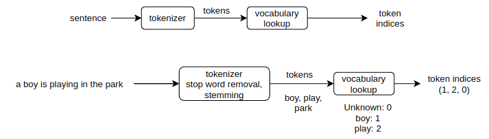
As you can see, tokenization rules and vocabulary work together and vary across domains. For examples, the tokenization rules and vocabulary for a medical . Therefore, NLP packages typically provide domain specific pipelines tokenization
Calculating BM25 statistics
Once we have the word embeddings, the next step is to use these word embeddings to create sentence embeddings. The obvious way to do this is to simply average the word embeddings for all the words that appear in a sentence. However this is likely not optimal because different words have different information content and embeddings of more important words should get a larger weight while creating the sentence embedding. The most popular way to calculate word importance is Term Frequency – Inverse Document Frequency (TF-IDF). TheTF-IDF value increases proportionally to the number of times a word appears in the document and is offset by the number of documents in the corpus that contain the word, which helps to adjust for the fact that some words appear more frequently in general (such as “the”). Many variants of TF-IDF exist and the cord19q ETL uses the BM25 variant. A comprehensive introduction and performance comparison of TF-IDF variants can be found in this paper.
The flowchart below shows the process of computing BM25 scores for each word.
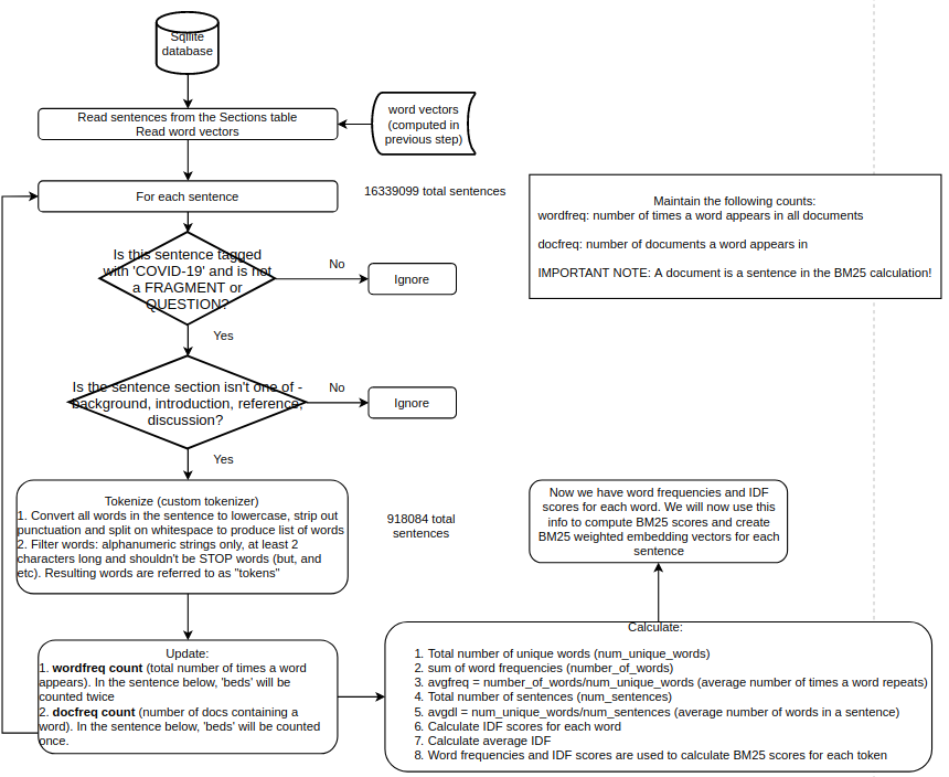
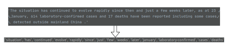
As mentioned earlier, only those sentences that come from documents tagged with the COVID-19 tag and aren’t a fragment or question are considered. The words in this filtered list of sentences are further filtered by removing stop words, words with fewer than 2 characters etc. Figure below shows this word filtering in action.
The resulting words are used to update the word frequency and document frequency counts which are then used to calculate the BM25 score for each word.
Output files
The parameters generated during the scoring process such as the word frequency and IDF (Inverse Document Frequency) frequency lists, average frequency, average IDF etc., are simply stored as a Python pickle file (scoring).
Number of embeddings and BM25 word counts
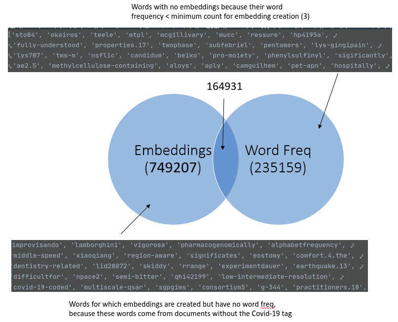
It is worth noting that the set of words for which embedding vectors are generated is not the same as set of words used to calculate BM25 statistics. There are two reasons for this:
- The filtering operations applied during embedding creation and computation of BM25 statistics are different. As shown in the flowcharts above, all documents are considered during embedding creation while only sentences from COVID-19 tagged documents and not belonging to certain sections (eg., introduction, background) are considered for scoring. This filtering leads to a significant winnowing out of sentences – from a total of 16339099 sentences in the corpus, only 917986 sentences are considered while computing BM25 statistics. Using the entire corpus during embedding creation makes sense because a large embeddings vocabulary helps makes out-of-vocabulary words less likely and also helps us exploit co-occurrence statistics from a larger corpus of documents.
- There are some words used during scoring that are are not in the embeddings vocabulary. This happens because of the mincount parameter passed to FastText during embedding creation. The word frequencies of these words is less than mincount.
The figure below shows a Venn diagram of these two sets of words along with some example of words that are in one set but not the other.
Calculating sentence embeddings
Once we have the word embeddings and the BM25 statistics for each word, we can easily calculate the BM25 weighted sentence embedding. Mathematically speaking, let  be the BM25 scores of the words in a sentence
  after any filtering operations such as stop word removal are applied. Let
  by the corresponding word embeddings. Then the embedding vector
  is:
is:

Here  is the number of words (after any filtering operations) in the sentence .
The flowchart below shows the process of creating sentence embeddings. The filtering operations applied on the sentences and words within a sentence are the same as before.
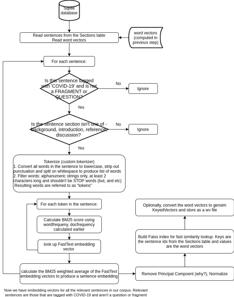
After the embeddings are calculated, the top principal component is removed. This is a common post-processing step in a NLP workflow. The intuition is that the highest variance components of the embedding matrix are corrupted by information other than lexical semantics. See this paper for more information
Once the sentence embeddings are calculated, we use Facebook AI’s Faiss library to store these embeddings on the disk. Faiss implements fast embedding lookup, so at query time, we convert the query into a sentence embedding and use Faiss to quickly find the top-n matches for the query.
Note that the embedding keys are the sentence ids, so at query time, we look up the sentence ids of the top-n matches, then we query the Sections table to get the document uid, and use the document uid to get the document info from the Articles table.
Output file
The sentence embeddings are saved to a embedding file using the write_index method of the Faiss library.
Finding the top-n matches for a given query
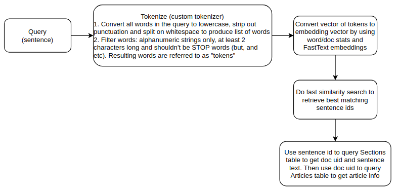
Finally, let’s consider how the sentence embeddings and BM25 scores are used to find the top-n matches for a user query. Given a query sentence, we first tokenize the query using the same rules used to tokenize the sentences in the corpus during embedding creation; use the BM25 scores and token embeddings to create an embedding representation for the query and then find the top-n sentences by using the lookup function in the Faiss library to do a fast similarity search. We then use the sentence ids of the top-n matches to query the sentence text and document uid from the Sections table followed by querying the Articles table to retrieve the article info using the document uid. The flowchart below shows this process.
Note that since the set of words used to compute BM25 scores and word embeddings don’t overlap, a query may contain words for which we have embeddings, but no BM25 statistics. For such words, average word and idf frequencies are used.
|
1 2 3 |
# Lookup frequency and idf score - default to averages if not in repository freq = self.wordfreq[token] if token in self.wordfreq else self.avgfreq idf = self.idf[token] if token in self.idf else self.avgidf |
This concludes this post. In the next post, we’ll look at using BERT models fine-tuned on a question-answering task to identify relevant answer spans to a query. The body text of the articles retrieved by the top-n matching articles returned by the lookup described above act as input to the BERT model.
Very insightful blogpost.Thank you for sharing the details.
I believe you have a typo in the section “Calculating sentence embeddings”. For the summation formula to be correct, it would seem that Wi would have to be the BM25score instead of “let Wi be the words in a sentence S” ?
Thank you very much, you are correct and I corrected the typo.