

In this post, I’ll describe my implementation and explanation of key elements of DeepAR, a probabilistic forecasting method based on autoregressive recurrent networks introduced by Amazon. DeepAR delivers accuracy improvements of ~15% over state-of-the-art methods and overcomes other shortcomings such as manual model selection, feature engineering and inability to handle count data.
The world is full of time series data. This data can be highly varied – it can be uni or multivariate, may have irregularly varying sampling rates, missing values and so on. A number of interesting problems with business significance can be formulated on time series data. Some examples are time series classification, prediction, forecasting and anomaly detection. Rather than attempting to provide an overview of these problems in this post, let me refer you to a couple of references I found very helpful. The first is the DeepAR paper and the tutorial for recently released GluonTS framework from Amazon that implements a variety of time series models. Section 3 of this tutorial provides an excellent, highly intuitive explanation and formulation of missing value imputation, forecasting, anomaly detection and other problems related to time series data analysis. Second reference is the time series workshop at ICML2019. I particularly recommend Prof. Yan Liu’s talk about “Artificial Intelligence for Smart Transportation” that discusses the range of algorithms used in traffic pattern analysis and forecasting.
This post will describe my PyTorch implementation of the probabilistic forecasting algorithm described in the DeepAR paper. The official implementation from Amazon is now available in the GluonTS library, however this library was not available when I started working on this project. While the availability of the GluonTS library makes this work somewhat redundant, I think it still adds value in the following ways:
- My implementation is in PyTorch, which is more widely used than MxNet, the deep learning library on which GluonTS is based.
- My implementation focuses on DeepAR, and should be easier to follow than GluonTS that implements a range of time series algorithms
- My implementation includes the deterministic model along with the probabalistic model. The deterministic model directly predicts the target values rather than the parameters of the likelihood function. The implementation of the deterministic model is easier to understand and debug than the likelihood model
- I provide preprocessing code and helpful visualizations for four popular datasets – NASDAQ100, SML2010, electricity and Beijing PM2.5 datasets
You should read the paper first to familiarize yourself with the key concepts involved in DeepAR. I’ll provide a brief overview here. We are given a number of time series  where
where  is the time series index and
  is the time index; and a set of covariates
  i.e., variables that have some relationship with the time series. The goal is to learn the conditional distribution of the future values of the time series, given its past and the covariates. For example, the Beijing 2.5PM dataset records the PM2.5 concentration (micrograms/cubic meter) at the U.S. embassy in Beijing, along with meteorological variables (the covariates) such as dew point, temperature, pressure, wind direction etc. Common sense suggests that these covariates have some bearing on the PM2.5 index, but we don’t know the mathematical model of this relationship. We also expect the PM2.5 index to exhibit seasonality, i.e., time dependence – the pollution index is likely to be lower during the night, over the weekend and higher during rush hour. Thus, it exhibits hourly and weekly seasonality, and likely monthly as well. Another example is the SML2010 dataset that contains the indoor temperature along with covariates such as relative humidity, sunlight intensity, outdoor temperature etc. Again, we expect all these covariates to influence the indoor temperature (the target series in this case), but we don’t know exactly how. We could rely on problem specific models for some of these dependencies (for example, a weather model for the pollution index), however it will be nice to have a single model that can automatically learn the correlation structure between different types of time series and can predict future values of the target series, without any manual feature engineering. This model should also handle missing values in some of the time series, time series of different lengths and irregular sampling rates. Out of these three, DeepAR can deal with the first two, but not the third (irregular sampling rates).
DeepAR further addresses the problem of jointly learning from time series with values spanning a wide range or where the distribution of values exhibits strong skew (power law distribution) or heavy tails (log normal distribution). It does so by incorporating a likelihood function that better models the statistical properties of the data. The paper discusses Gaussian likelihood for real-valued data and negative binomial for count data. Since the datasets used in my experiments contain real valued data, my implementation covers Gaussian likelihood only.
Table of Contents
Model
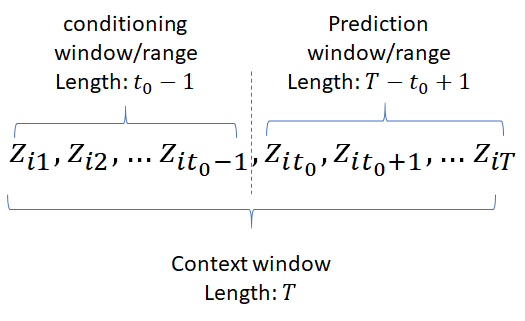
Denoting the value of the time series at time by  , the goal is to model the conditional distribution of the future of each time series
 ![[z_{i,t_0}, z_{i,t_0+1},\hdots,z_{i,T}] :=\mathbf{z}_{i,t_0:T}](https://www.telesens.co/wp-content/ql-cache/quicklatex.com-da5f95f2c40e00204e60c92fbf8dedb9_l3.png "Rendered by QuickLaTeX.com") given its past
given its past ![[z_{i,1}, z_{i,t_0-2},\hdots,z_{i,t_0-1}] :=\mathbf{z}_{i,1:t_0-1}](https://www.telesens.co/wp-content/ql-cache/quicklatex.com-89a37d45c98625ab86403fcb86dcd608_l3.png "Rendered by QuickLaTeX.com") ,
,

 denotes the time point from which we assume to be unknown at prediction time and
  are covariates assumed to be known for all time points. During training, multiple training instances are generated by selecting windows with different starting points. The “past” and “future” terms are with respect to the starting point of each training sample. To avoid confusion, the time ranges
 ![[1, t_0-1]](https://www.telesens.co/wp-content/ql-cache/quicklatex.com-ebf3d801bd4df91b6decb80609d1142a_l3.png "Rendered by QuickLaTeX.com") and
and ![[t_0, T]](https://www.telesens.co/wp-content/ql-cache/quicklatex.com-1bdb51b84c44abff3d9559c26b484f6b_l3.png "Rendered by QuickLaTeX.com") are called conditioning range and prediction range respectively, instead of past and future.
are called conditioning range and prediction range respectively, instead of past and future.
The probabilistic model outputs the parameters of the likelihood factors which can be used to calculate the probability of the target sequence:

here  is the output of the autoregressive neural network (stacked LSTM in our case), whose function
  is parameterized by
  . For a stacked LSTM, would be the parameters of the various weight matrices (input-hidden, hidden-hidden etc) of the LSTMs. The likelihood
  is a fixed distribution, whose parameters are given by a function
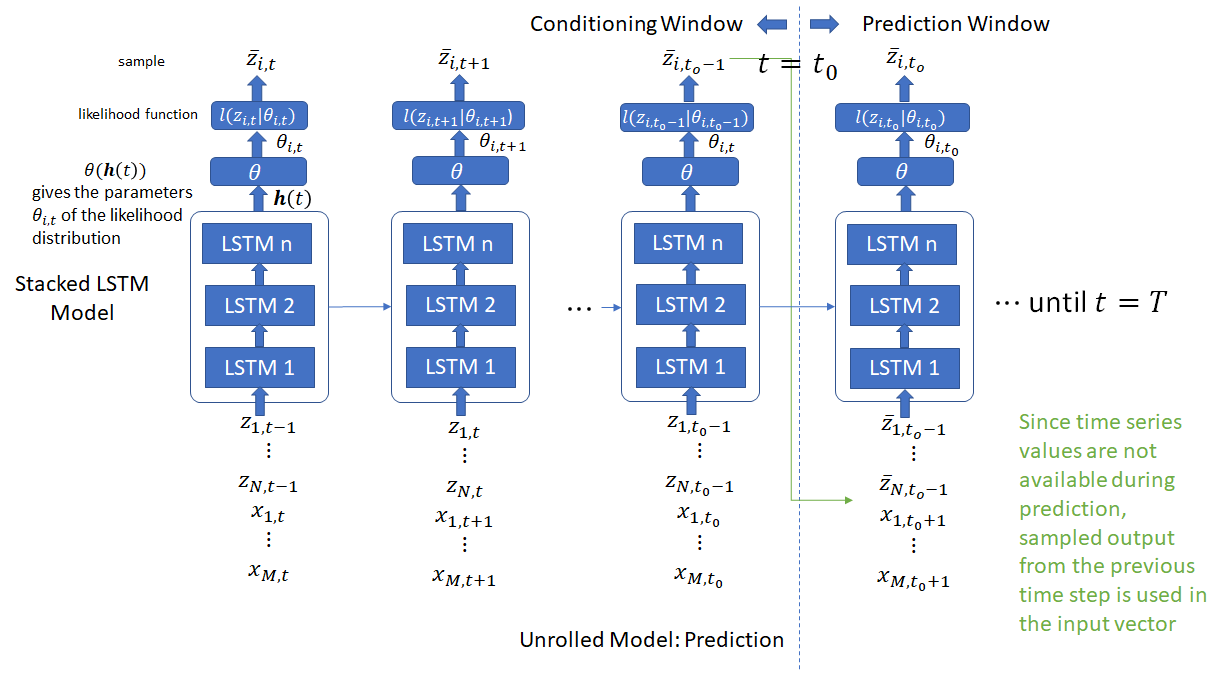
  of the network output . For the Gaussian likelihood, these would be the mean and variance of the Gaussian distribution. The model is autoregressive because it consumes the observation at the last time step as an input and recurrent because the hidden and cell states of the LSTM units from the last time step are fed back as input in the next time step. The figure below shows the operation of the network at one time step. Note that the std deviation output is fed into a softplus unit to ensure positivity before the loss calculation.
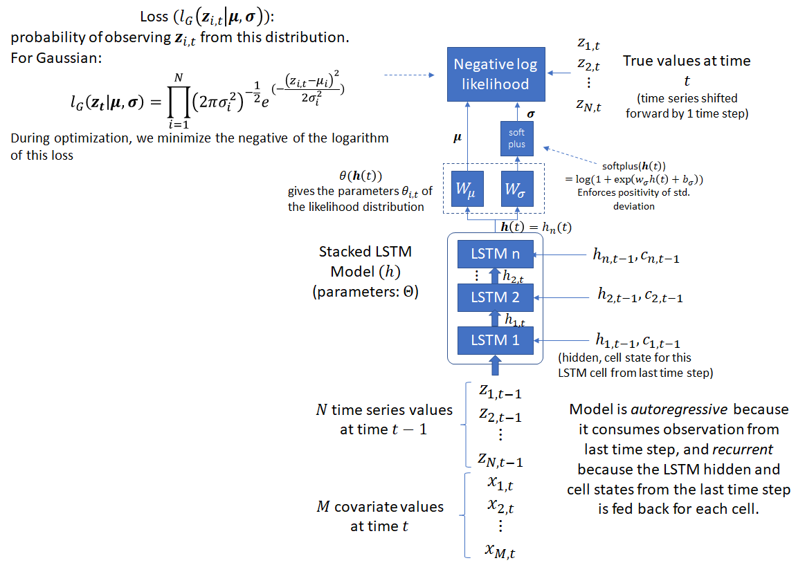
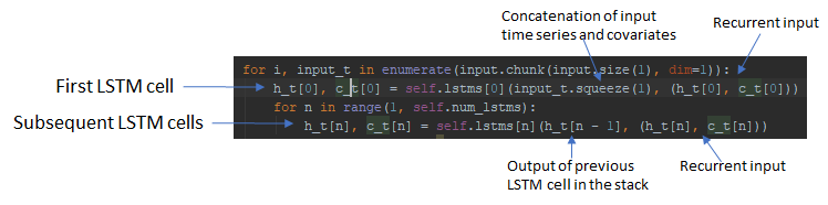
Note that the DeepAR paper uses the letter to refer to the LSTM outputs, which can also refer to the LSTM hidden state. In Pytorch, the DL library I use for the experiments described in this post, the output of a LSTM cell are , the hidden state and  , the cell state. For a stacked LSTM model, the hidden state is passed to the next LSTM cell in the stack and and from the previous time step are used as the recurrent input for the current time step, along with the output of the previous LSTM cell in the stack (except the first LSTM cell, which takes as input the concatenated input time series and covariates).
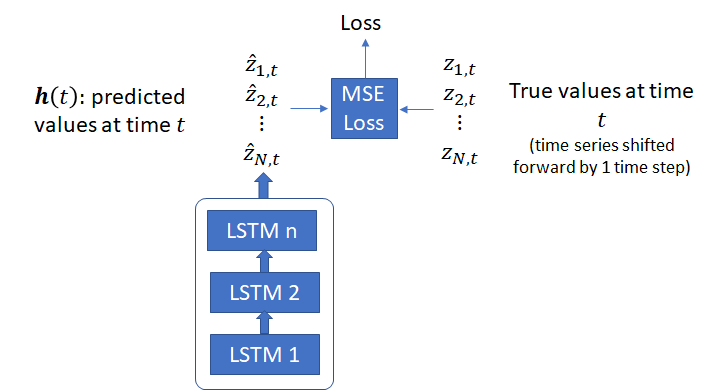
In addition to the likelihood model, I have also implemented a simpler version, where the model predicts the target time series values directly, rather than the parameters of a distribution. In this model, a distance function such as Mean Square Error (MSE) between the model output and the actual target values can be used as the loss function. In the results shown below, I’ll show the output of both models.
DeepAR uses previous time step values to condition the model for the current time step. These values are available in the conditioning range during both training and prediction. For the prediction range, one must distinguish between training and prediction. During prediction, the time series values in the prediction range are not available (because that’s what we are trying to predict). Therefore, samples from the likelihood function (whose parameters are predicted during the previous step) are used as the input values for the current time step. For the deterministic model, the model output for the previous time step can be used directly.
During training, we have three options for the prediction window:
1- Simply use the actual time series values for the previous time step. This is possible because these values are available for the prediction range during training. Doing so presents a easier learning task for the model, however introduces a discrepancy between the prediction and training task
2- Use samples from the likelihood (or model output for the previous time step for the deterministic model), just as during prediction. This presents a more difficult learning task because the errors in model parameters during one time step will propagate to future time steps.
3- Use a combination of the two – for example, scheduled sampling where option 1 is used with probability  (option 2 with probability
  ). The probability is lowered as training progresses. The intuition is that as training progresses, the model will learn to make better predictions making it safer to use samples from model predicted likelihood function, keeping the difficulty of the training task relatively level.
The DeepAR paper recommends using option 1 because option 2 slows down convergence. In my implementation, I used option 2, mostly because this keeps the training and prediction code identical. The covariates are assumed to be available for all time steps during training and prediction, so no special consideration is needed.
If you find this discussion a bit convoluted, ponder it for a while and it will start making sense 🙂
Encoder-Decoder architecture
DeepAR paper provides an interesting analogy between the encoder-decoder architecture used by seq-to-seq translation systems used in machine translation, video captioning etc. These systems use recurrent cells (LSTM/GRU/RNN) to encode (summarize) the input sequence into a context vector which is used by the decoder to generate the target sequence. In these systems, typically the encoder and decoder use different architectures and do not share weights. DeepAR uses the same architecture for both the encoder and decoder with weight sharing. In fact, there is no distinction between the encoder and decoder model – only the inputs are different. In the conditioning range, the actual time series values are used while in the prediction range, the samples from the output distribution are used during prediction. For training, one could also use the actual time series values or samples from the output distribution, as discussed above. The LSTM output at time  (for each LSTM cell in the stacked LSTM model) acts as the context vector and initializes the hidden state of each LSTM cell for the first time step during decoding.
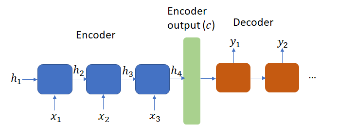
Encoder-Decoder architecture presents a difficult learning task as the encoder must compress all necessary information about a source sequence into a fixed length vector. To address this issue, Bahdanau et. al. introduced the attention mechanism (in a machine translation context) that encodes the input sentence into a sequence of vectors and uses a linear combination of these vectors while decoding the translation. Researchers have applied the attention mechanism to time series modeling as well. See this for example. Adding the attention mechanism to DeepAR could be an interesting extension.
Creating Batches
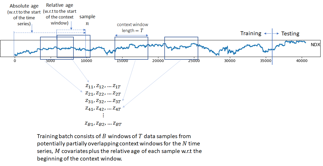
Batch element are generated by selecting windows with different starting points from the original time series. The total number of samples as well as the relative length of the conditioning and prediction ranges are fixed for all batches. DeepAR recommends adding the relative age of time samples w.r.t the beginning of the context window and the absolute age w.r.t the beginning of the time series to the covariates. In my implementation, I only use the relative age. Adding the absolute age didn’t make a significant difference in my experiments. To make this more concrete, lets say we have  time series,
  covariates, batch size is
  and the size of the context window is
  , then each batch will be a tensor of dimensions
  , where the last 1 corresponds to the relative age. Other time covariates indicating seasonality such as hour-of-day for hourly data, day-of-week for weekly data are also added to the covariates. DeepAR also adds an embedding vector (jointly trained with other model parameters) corresponding to item category for large datasets and item identity for smaller datasets. My implementation does not use item embeddings.
The first two dimensions of a batch are shown in the diagram below.
Handling Scale
I use a different scaling mechanism than what is described in the DeepAR paper (mostly because I didn’t quite understand their scaling method and mine is simpler and performs well). For each batch element, I subtract the mean and divide by the range. Predicted values are then converted back to the original scale by applying the inverse transform. When the model outputs the likelihood parameters (mean and std. deviation of the Gaussian distribution), the invert scale for the mean is the same as before, and the standard deviation is scaled by the square root of the range. This is because for a random variable  with mean
  and standard deviation
  , the mean and std. deviation of the transformed variable
  is
is  and
and  .
.
Code Organization
All of my training and testing code, and the preprocessed csv files for the SML2010, NASDAQ100 and PM2.5 datasets are here
I leverage the Pytorch dataloader infrastructure to create batches. the Dataloader class needs an instance of the Dataset class that knows how to return data for a given index and an instance of the base Sampler class whose subclasses provide different ways to iterate over indices of dataset elements. For example, the RandomSampler class samples elements randomly, SequentialSampler samples sequentially. So the main task is to write Dataset classes that know how to read chunks for the different Datasets I use in my experiments. I do this as follows:
- Pytorch Dataset
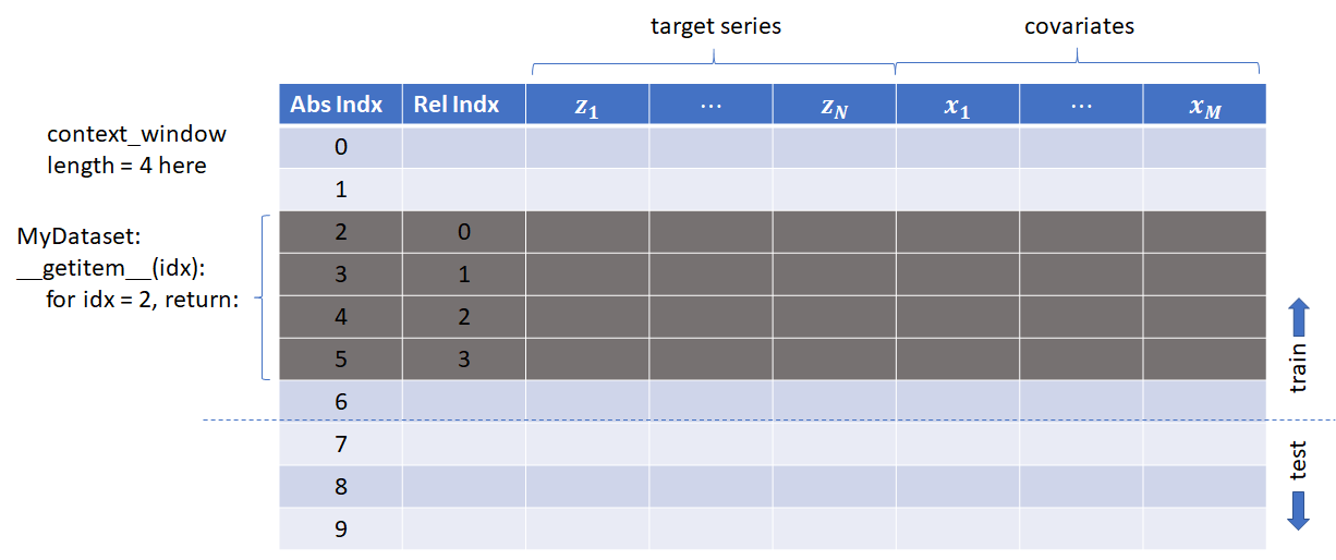
- MyDataset (very imaginative, I know..): implements the __len__ method which returns the dataset size and __getitem__ that returns a portion of the dataset corresponding to the index passed as a parameter and appends the relative (and absolute, if needed) time index.
- electricity_dataset
- NSDQ100_dataset
- etc
- MyDataset (very imaginative, I know..): implements the __len__ method which returns the dataset size and __getitem__ that returns a portion of the dataset corresponding to the index passed as a parameter and appends the relative (and absolute, if needed) time index.
For each dataset, there is a subclass of MyDataset that reads the csv file corresponding to that dataset in its __init__ function and creates a data structure in the format shown below. During each __getitem__ call, MyDataset then returns chunks from this data structure.
The code is organized as follows:
- /data: contains the preprocessing scripts and the preprocessed csv files for the datasets. The csv for the Electricity dataset is not included because it is >100 MB. However you can download the original Electricity dataset from https://archive.ics.uci.edu/ml/datasets/ElectricityLoadDiagrams20112014 and run the electricity_preprocess.py script on it to generate the csv file. The preprocessing scripts read the original data as pandas dataframe, format the dates, drop unnecessary columns and save the processed data into csv files that can be read during training. It also contains the config files for each dataset that describes the number of target time series, covariates, context window length, conditioning window length, number of epochs and other variables.
- /dataset: contains the dataset classes for the various datasets as explained above
- /models: contains the implementation of the deterministic and likelihood models
- /utils: utils.py that contains helper functions to split up a batch into input, target and covariates, apply per batch scaling, inverse scaling and implementation of metrics (RMSE, NRMSE etc.)
- example1.py: implements deterministic training
- example1-prob.py: implements probabilistic training
- prediction.py: shows how to load a model and run prediction. For convenience, I provide pretrained models for the BeijingPM2.5 dataset for different number of covariates and epochs. You should be able to directly run the prediction.py script with no arguments to generate the results shown here for that dataset.
Datasets
I used the following datasets in my experiments:
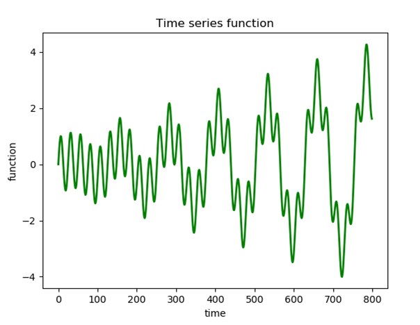
- Amplitude modulated mixture of sine waves (
 )
) - SML2010: consists of weather related parameters such as temperature, relative humidity, sunlight intensity collected from a monitor system mounted in a house
- Beijing PM2.5: consists of PM2.5 data of U.S. Embassy in Beijing along with meteorological data from Beijing International Airport
- NASDAQ100: subset of the full NASDAQ 100 dataset consisting of 105 days’ stock data for 81 stocks starting from July 26, 2016 to December 22, 2016. Each day contains 390 data points except for 210 data points on November 25 and 180 data points on December 22.
- Electricity: Household electricity consumption by 370 households in Portugal
The table below shows the number of time series in each dataset along with the number of data points.
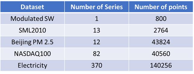
For the SML2010 and Beijing PM2.5 datasets, the target time series is the indoor dining room temperature and the PM2.5 index respectively. Other time series are used as covariates. This makes sense because for the Beijing PM2.5 dataset, we expect the PM2.5 level to depend on the meteorological data such as temperature, pressure, wind direction but we don’t know the nature of the relationship. We also expect the PM2.5 level to have seasonal variation – for example lower levels over nights/weekends than during the day/week. This is exactly the scenario that DeepAR is expected to model well.
For NASDAQ and Electricity datasets, the time series are separate instances of the same variable – stock indices in case of NASDAQ100 and electricity consumption for the electricity dataset. For these datasets, there isn’t a natural choice for the target variables and the covariates and we can pick any subset of variables as the target variables and covariates. For the NASDAQ dataset, I used the NSDQ composite index as the target and 70 out of the 81 stock indices as the covariates. For the electricity dataset, I used 100 out of the 370 electricity time series as the targets and the time variables – day-of-week (DOW), hour and minute as the covariates.
Below, I’ll show some sample data and cross correlation heatmaps that provide intuition about the time series in the datasets.
Amplitude modulated mixture of sine waves
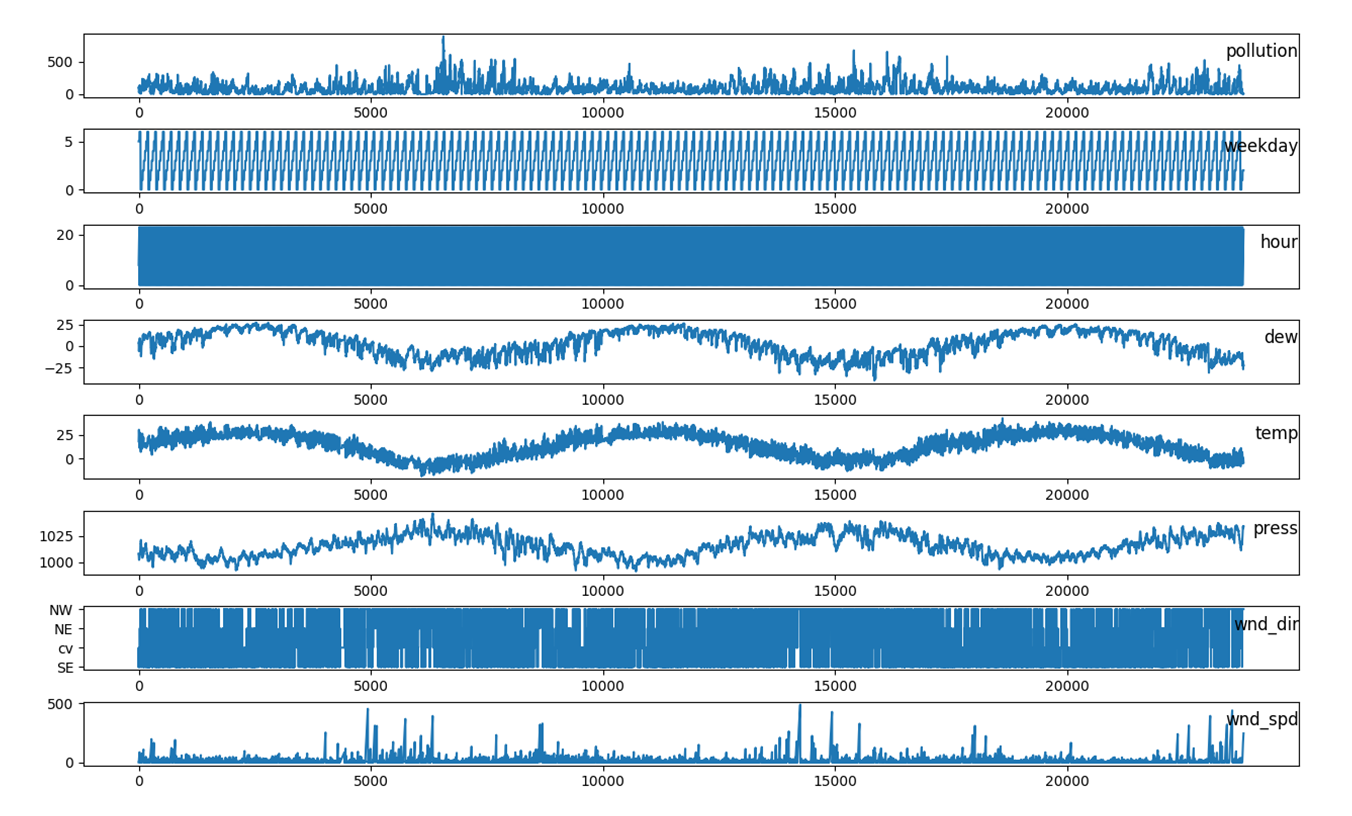
Beijing PM 2.5 Dataset
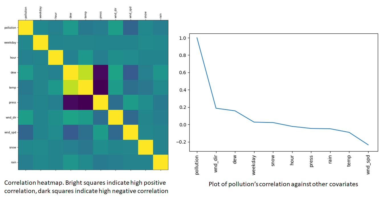
From these plots, we can see that our variable of interest, PM2.5 concentration has some correlation with the covariates, so we expect the inclusion of covariates to be helpful in making PM2.5 predictions. Furthermore, some covariates such as dew and temperature have a higher cross-correlation than others. This suggests that some of these covariates could be dropped as the information in these covariates can be captured by including only a smaller subset.
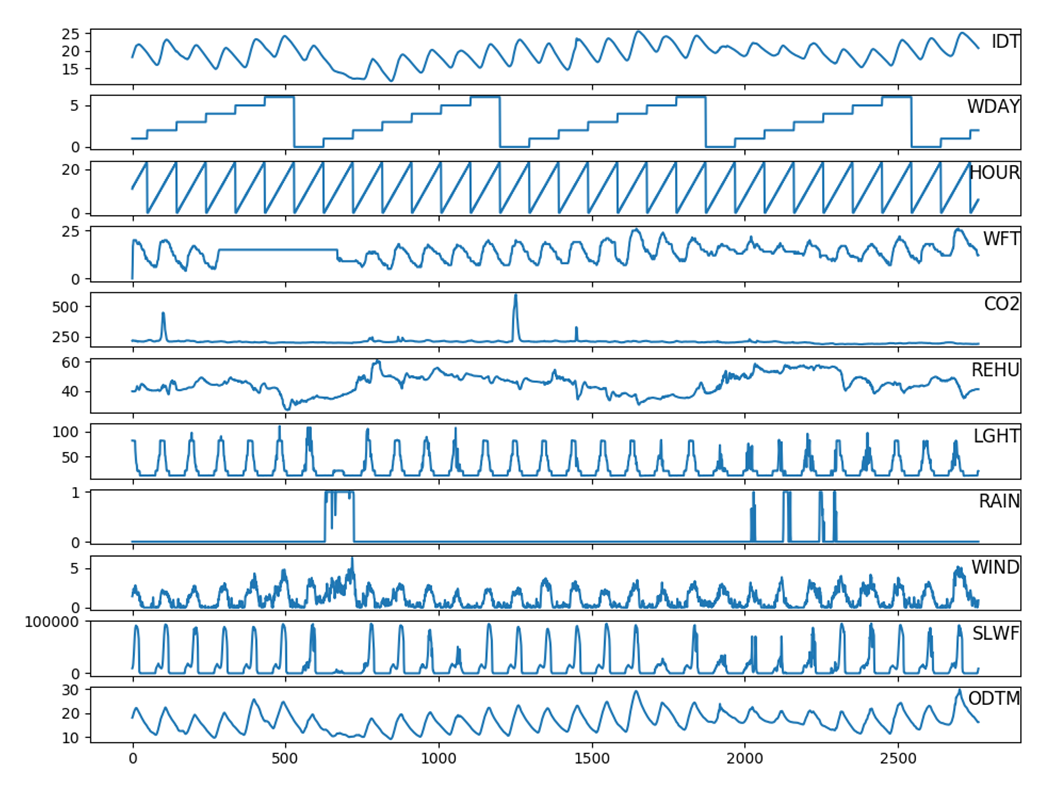
SML2010 Dataset
The SML2010 Dataset consists of 24 time series. Out of these, I selected the following 13 time series.
- IDT: Indoor Temperature (Dining Room)
- WDAY: Weekday (0-6)
- HOUR: hour
- MIN: minutes
- WFT: Weather forecast temperature (degree Celsius)
- CO2: Carbon dioxide in ppm (dinning room)
- REHU: Relative humidity (dinning room), in %
- LGHT: Lighting (dinning room), in Lux
- RAIN: Rain, the proportion of the last 15 minutes where rain was detected (a value in range [0,1])
- WIND: Wind, in m/s
- SLWF: Sunlight in west facade, in Lux
- ODTM: Outdoor temperature, in (degree Celsius)
- ODRH: Outdoor relative humidity, in %
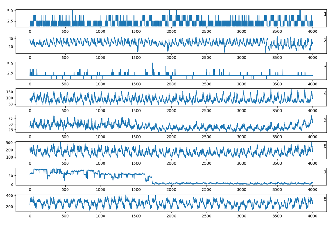
Some of these time series are plotted below. The scales for the series are clearly very different.
The cross-correlation heatmap is shown below. Indoor temperature in the dining room – our target variable has higher correlation with the covariates than we saw earlier with the PM2.5 dataset. 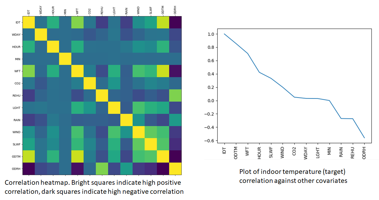
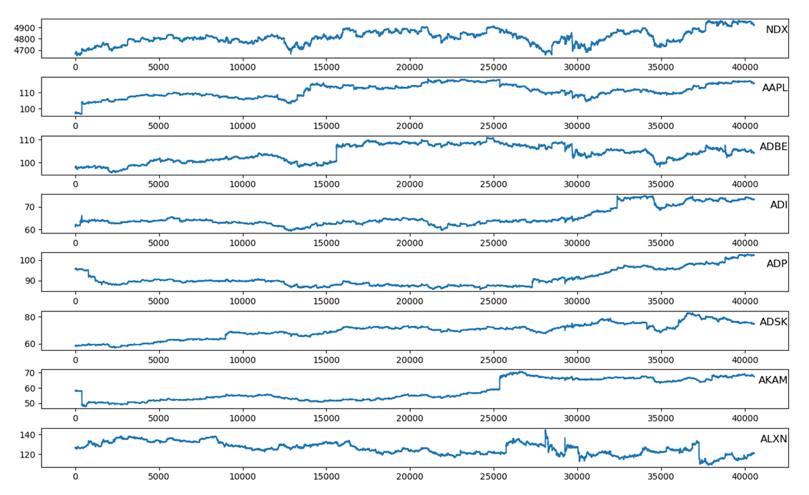
NASDAQ 100 Dataset
Plots for some of the stock indices in the NASDAQ dataset are shown below. Notice that because of the global upward trend in the time series, calculating the mean and range for the entire time series will not be optimal. Batches from earlier in the time series will undershoot the mean while later batches will overshoot. This is why it is better to apply per-batch normalization for each time series
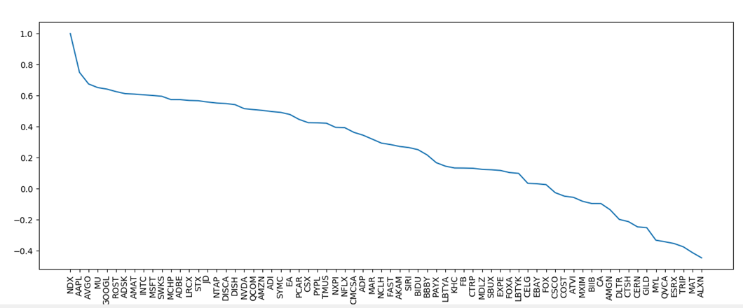
The stock indices sorted by correlation with NDX (NASDAQ composite index) in decreasing order are shown below. As expected, NDX being a tech dominated index is more strongly correlated with tech companies with large market cap.
Electricity Dataset
Finally, the figure below shows some of the time series from the electricity dataset. As expected, the plots show a high degree of seasonal variation and considerable variability between each other.
Results
Below, I’ll provide the results for the four datasets listed above for both the deterministic model, that predicts the target values directly and the likelihood model that predicts the parameters of the normal distribution. I’ll show the target values in red color and the predicted values in the conditioning range in green and in the prediction range in dashed green. For the likelihood model, I’ll also show the  and
and  plots for ease of visualization.
For the direct model, I’ll report Root Mean Square Error (RMSE), Mean Average Error (MAE), Normalized RMSE (NRMSE) and Normalized Deviation (ND). These are defined as follows:
- RMSE =

- NRMSE =

- MAE =

- ND =

Note that only the values in the prediction window are considered in these calculations. The averages are calculated over all target time series and time steps in the prediction window.
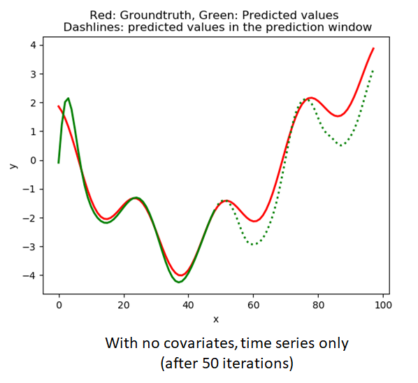
Amplitude modulated mixture of sine waves
This is the simplest test case with no covariates except for the relative age (time index of a sample w.r.t the beginning of the context window). I ran the model with and without the relative time index to see if the model benefits from the relative age. As the results below show, the inclusion of the relative age appears to help.
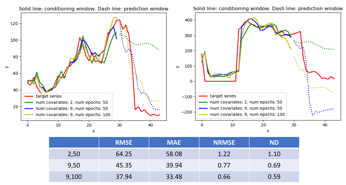
Beijing PM 2.5 Dataset
For this dataset, the task is to predict the hourly PM2.5 values given the meteorological conditions. I used a context window of length 45 hrs, conditioning window length 30 hrs and prediction window length 15 hrs. I wanted to investigate two issues:
- Does the inclusion of meteorological covariates aid in learning a better model over just the seasonal (hour, day-of-week) covariates? To investigate this, I ran the model with just the seasonal covariates and then included some of the meteorological covariates. As shown in the results below, the inclusion of the meteorological covariates appears to help
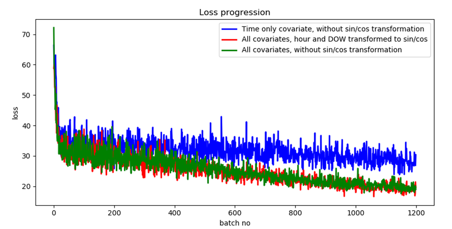
- Encoding time variables such as minutes/hours/day-of-week into a sequence of increasing numbers can distort the cyclical relationship inherent in periodic time variables. For example, 11PM is closer to 1AM in time than 5AM is to 1 AM. However, if we encode hours as numbers from 0-23, then 11 PM (encoded by 23) would appear to be farther from 1AM (1) than 5AM (5). Same logic applies to encoding day-of-week by numbers from 0-6. To address this issue, people have proposed encoding time variables into dual sine and cosine features which correctly captures the cyclical relationship. See this post for an example.
I found that converting the time variables into sin/cos features doesn’t make a significant impact. The plot below shows the loss progression with only the time covariate (blue plot), all covariates with hour and day-of-week converted into sin/cos (red plot) and all covariates without the sin/cos conversion (green plot). It is clear that while the inclusion of other covariates helps, the conversion to sin/cos doesn’t. The conversion also doubles the number of cyclical covariates, because two covariates series (sin() and cos()) are generated from each such covariate, thus increasing model complexity. In the rest of my experiments, I do not use the sin/cos conversion.
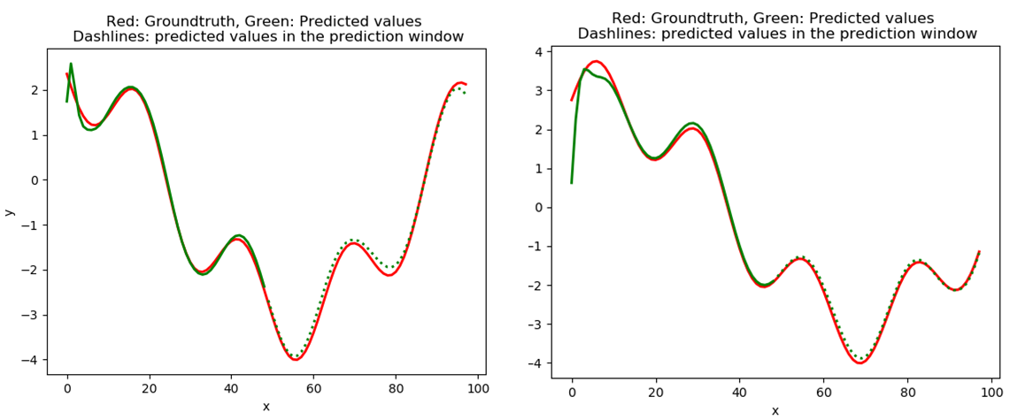
The plots below show the effect of including the meteorological covariates and running the model for larger number of iterations. The model’s predictions get better as additional covariates are included and the model is trained for longer.
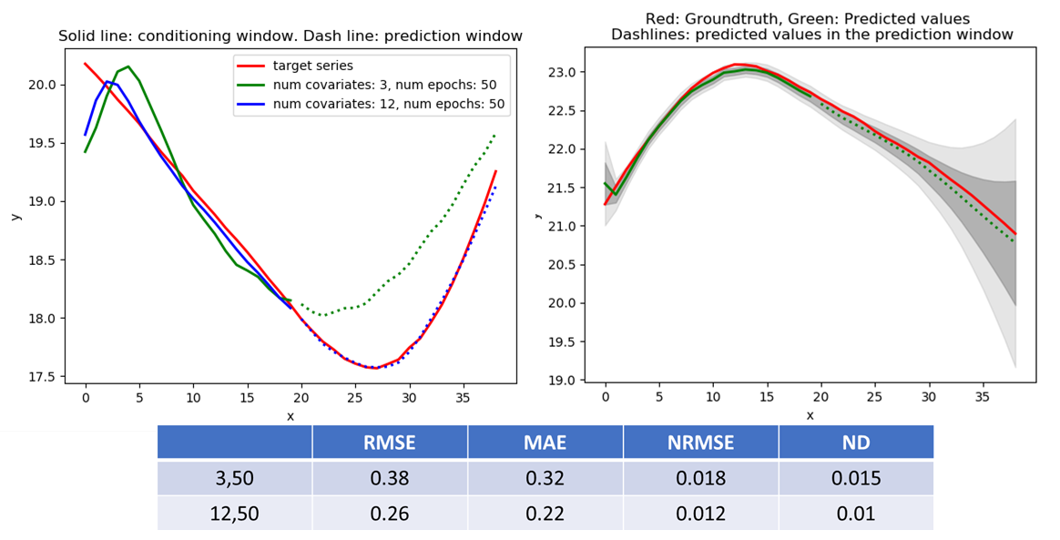
SML2010 Dataset
The results for the SML2010 dataset, along with a prediction example for the direct and likelihood based model are shown below. I used a context window length = 40 with conditioning window = 20 and prediction window = 20. Again, inclusion of additional covariates helps with making better predictions. The plot on the right shows the result of the likelihood model. I use the mean value as the model prediction and  and
and  plots are shown in dark gray and light gray. The true target values (shown in red) stay comfortably within the model prediction range.
NASDAQ 100 Dataset
The NASDAQ 100 dataset consists of stock price information for several stock tickers. It doesn’t have any natural covariates. In my experiment, I used NDX (the NASDAQ composite index) as the target, and 70 out of the 81 stock tickers as the covariates. I used a context window length = 40 with conditioning window = 20 and prediction window = 20. The prediction results for the direct and likelihood model are shown below.
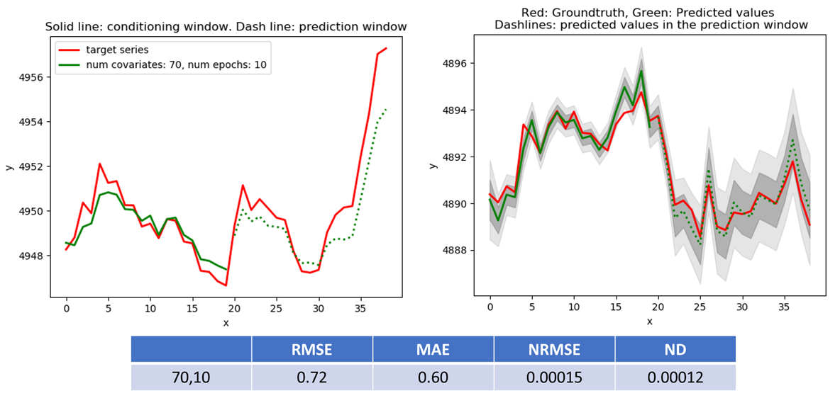
The RMSE and MAE metrics for the SML2010 and NASDAQ 100 datasets compare favourably with the results of the DA-RNN (RNN with dual-stage attention) model described in this paper.
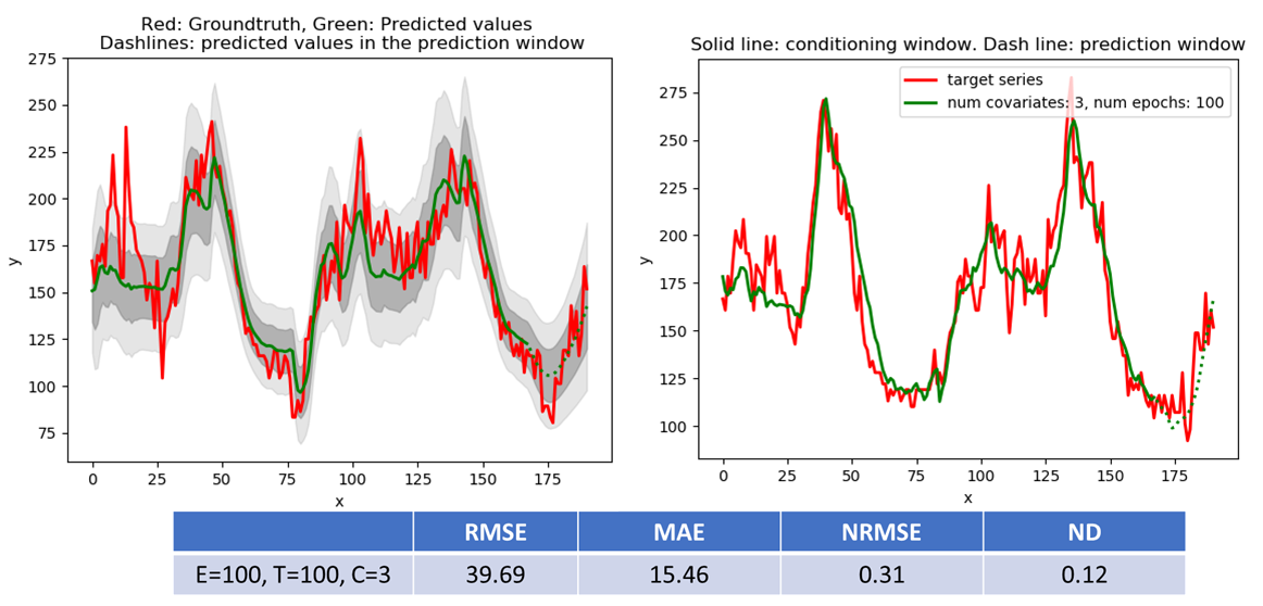
Electricity Dataset
Like the NASDAQ dataset, the electricity dataset also doesn’t have natural covariates – i.e., factors with which electricity consumption may be correlated. An example of such covariates is water consumption per household, which could be correlated with electricity consumption through household size. There are three seasonal covariates – minutes, hours and day of week. I used 100 of the 370 available time series as the target, the three seasonal covariates, context window length = 192 with conditioning window = 168 and prediction window = 24. Some results are shown below. The ND and NRMSE compares favourably with the results shown in the DeepAR paper. Their RMSE is equivalent to my NRMSE.
Conclusion
I hope you found this post and associated code helpful in developing intuition about how autoregressive, recurrent machine learning models such as DeepAR are used in time series data analysis. I welcome any comments, feedback about this post and pull requests for the code.
Thanks for sharing Ankur! If you had used MAE instead of MSE as the loss for the deterministic case, you should have obtained the same P50 values of the probabilistic case? (since you are using Gaussian likelihood)
I would love to see the implementation of a deterministic DeepAR (with flexible loss functions) in GluonTS.
Did you compare your Nasdaq 100 predictor with a contemporaneous regression on a simple average of 70 stocks?
The latter is simply d% NDX(t) ~ a + b * d% x(t), where d% is percentage change and x(t) is a simple average of 70 stocks. You could go for cap weighted average, but simple average should be good enough. I’d be surprised if this regression did worse than the ML model.
Stock indices are pretty much impossible to truly forecast, especially on such a short horizon. However, in your case if you assume you know prices of 70 tickers, in reality you already have NDX index too, because it’s a simple calculation based on the prices of 100 tickers. Hence, a simple average of 70 tickers should be an excellent proxy for NDX, especially if the tickers are traded in NASDAQ themselves.
Thanks for the comment and your observation is absolutely correct. I did not compare my forecast with that predicted by a simple model such as the one you suggest. As you say, a simple model is likely to perform well when price information for other similar stocks is already available. I included the Nasdaq dataset mostly to compare my results with other published results. The utility of DeepAR style ML based models is better for datasets such as Beijing PM where the correlation structure between the target variables and covariates is complex and difficult to model and reliable forecasts exist for some of the covariates – for example the temperature forecast in case of the Beijing PM dataset. In this scenario, the model can learn the complex correlation structure between the target variables and the covariates from past observations and then use the learned model and covariate forecasts to make better predictions for the target variables. The application of DeepAR to the Beijing PM dataset shows that the technique works.
I’d be curious to see how DeepAR stacks up against FB’s Prophet. They seem to address the same issue: mass time series forecasting, commoditizing the domain. My experience with Prophet was that it’s prone to following the recent trend and underestimating the mean reversion. I wonder if DeepAR suffers from the same problem.