Efficiently Computing the Fisher Vector Product in TRPO

The purpose of this post is to provide math proofs and clarify some implementation details in the recently introduced reinforcement learning method called “Trust Region Policy Optimization” (TRPO). Standard policy gradient methods try to find a policy that maximize expected rewards by solving the optimization problem:

(1) $\begin{equation*} \begin{align} \max_\theta J(\pi_\theta) = E_{\tau \sim \pi_\theta}[\sum_{t=0}^\infty \lambda^t r_t ] \end{align} \end{equation*}$

This problem is solved by performing stochastic gradient ascent on the policy parameters. For more details, refer to the excellent lecture slides on “Advanced Policy Gradient Methods” as part of the Reinforcement Learning class at UC Berkeley. As a side note, I applaud the recent trend in academia to make class lecture notes at top universities available to everyone. This, accompanied by a similar trend in research to make code for new machine learning algorithms available is making it possible for anyone willing to put in the time and effort to master latest advances in machine learning. This spirit of openness will make the field accessible to talented minds all over the world who may lack the means to go to Stanford or Berkeley and help address the growing mismatch between the supply of and demand for machine learning practitioners.

The problem is that this approach offers no principled way to choose the right step size. If the step size is too big, the optimization may miss the minimum. If the step is too small, progress may be very slow. Standard machine learning methods address this problem by using automatic learning rate adjustment such as the Adam optimizer. However as illustrated in the lecture slides, the problem with the policy gradient methods is that small changes to the policy network parameters can cause unexpectedly large changes in the policy output (action probabilities).

TRPO offers a mathematically principled approach to this problem by re-framing the optimization problem as a constrained optimization whose solution is guaranteed to result in an improved policy. For details, refer to the lecture slides and the original TRPO paper. There are many PyTorch implementations of TRPO available. I’m using this one – https://github.com/Khrylx/PyTorch-RL. PyTorch is my favorite machine learning library. Someone I know recently said – “Looking at TensorFlow code gives me a headache, using PyTorch makes me smile”. I agree with that sentiment :-).

Parts of this code took me considerable effort to understand, particularly the proof of the fast method to calculate the Fisher vector product and its PyTorch implementation. The main purpose of this post is to offer explanations for the math and code so that it will be easier for you to follow. I’ll focus on the TRPO step and assume you already understand how to calculate value functions, compute advantages and other standard reinforcement learning techniques that are not specific to TRPO.

The constrained optimization problem solved in TRPO is stated as follows:

(2) $\begin{equation*} \begin{align} \pi_{k+1} = arg \max_\pi L(\pi) \text{ st } D_{KL}(\pi, \pi_k)\leq \delta \end{align} \end{equation*}$

Here $D_{KL}(\pi, \pi_k)$ is defined as

(3) $\begin{equation*} \begin{align} D_{KL}(\pi, \pi_k)= \sum(\pi_k)\log\frac{\pi_k}{\pi} \end{align} \end{equation*}$

$\pi_k$ refers to the output of the network (at the $k^{th}$ iteration) with parameters $\theta_k$ , representing a probability distribution over the action space. $\pi$ is short for $\pi_\theta$ , the subscript may be dropped in some places below as the dependence of the policy on the network parameters is implicit. Since $\theta_k$ and hence $\pi_k$ is fixed (at the end of iteration $k$ ), the only variable in the formula above is $\pi$ . Therefore, while calculating derivatives using autograd, we must detach $\theta_k$ from the computation graph. The summation is over the elements of the $M \times 1$ dimensional $\pi$ vector, the output of the policy network.

 def get_kl(self, x):
        action_prob1 = self.forward(x)
        # calling .data detaches action_prob0 from the graph, so it will not be part of the gradient computation.
        # Also, starting PyTorch 0.4, the Variable wrapper is no longer needed. 
        action_prob0 = Variable(action_prob1.data)
        kl = action_prob0 * (torch.log(action_prob0) - torch.log(action_prob1))
        return kl.sum(1, keepdim=True)

def get_kl(self, x):

action_prob1 = self.forward(x)

# calling .data detaches action_prob0 from the graph, so it will not be part of the gradient computation.

# Also, starting PyTorch 0.4, the Variable wrapper is no longer needed.

action_prob0 = Variable(action_prob1.data)

kl = action_prob0 * (torch.log(action_prob0) - torch.log(action_prob1))

return kl.sum(1, keepdim=True)

The loss function is defined as

(4) $\begin{equation*} \begin{align} L(\pi) = E_{\tau \sim \pi_k}[\sum_{t=0}^\infty \gamma^t \frac{\pi(a_t|s_t)}{\pi_k(a_t|s_t)}A^\pi(s_t, a_t)] \end{align} \end{equation*}$

The gradient of this loss function wrt to the policy parameters $\theta$ is:

(5) $\begin{equation*} \begin{align} \nabla_\theta L(\pi)|\theta = \theta_k = E_{\tau \sim \pi_k}[\sum_{t=0}^\infty \gamma^t \nabla_\theta \log\pi_\theta(a_t|s_t)|_{\theta = \theta_k} A^{\pi_{\theta_k}}(s_t, a_t)] \end{align} \end{equation*}$

This gradient can be readily computed as the state-action sequence under the current policy is already available. The code to calculate the loss and gradient is shown below. We compute the policy gradient both using autograd and the formula above.

######
    # Run forward pass on a state to get the probability distribution over actions
    action_prob = policy_net.forward(states[0])
    # Let's look at the first action
    log_prob = torch.log(action_prob[actions[0]])
    # detach from the graph so we don't compute derivative wrt this
    fixed_log_prob = log_prob.detach()
    # Formula for loss. Need to exponentiate the log prob to get prob. 
    # Advantages have been computed earlier in the program
    action_loss = Variable(advantages[0]) * torch.exp(log_prob - fixed_log_prob)
    # Compute derivative using autograd
    grad1 = torch.autograd.grad(action_loss, policy_net.parameters(), retain_graph=True)
    # grad_flat will be a vector K*1, where K is the total number of parameters
    # in the policy net. 
    grad1_flat = torch._utils._flatten_dense_tensors(grad1)
    # Now compute derivative using policy gradient formula
    _grad2= torch.autograd.grad(log_prob, policy_net.parameters())
    _grad2_flat = torch._utils._flatten_dense_tensors(_grad2)
    grad2 = advantages[0]*grad2_flat
    # verify grad2 == grad1
#######

######

# Run forward pass on a state to get the probability distribution over actions

action_prob = policy_net.forward(states[0])

# Let's look at the first action

log_prob = torch.log(action_prob[actions[0]])

# detach from the graph so we don't compute derivative wrt this

fixed_log_prob = log_prob.detach()

# Formula for loss. Need to exponentiate the log prob to get prob.

# Advantages have been computed earlier in the program

action_loss = Variable(advantages[0]) * torch.exp(log_prob - fixed_log_prob)

# Compute derivative using autograd

grad1 = torch.autograd.grad(action_loss, policy_net.parameters(), retain_graph=True)

# grad_flat will be a vector K*1, where K is the total number of parameters

# in the policy net.

grad1_flat = torch._utils._flatten_dense_tensors(grad1)

# Now compute derivative using policy gradient formula

_grad2= torch.autograd.grad(log_prob, policy_net.parameters())

_grad2_flat = torch._utils._flatten_dense_tensors(_grad2)

grad2 = advantages[0]*grad2_flat

# verify grad2 == grad1

#######

Here $\tau$ is the state action sequence generated by following $\pi_k$ , the policy at time step $k$ . The goal is to find the optimal new policy $\pi$ that is guaranteed to decrease the loss function

Expanding the loss function and the KL distance using Taylor series expansion around $\theta_k$ ,

(6) $\begin{equation*} \begin{align} L_{\theta_k}(\theta) = L_{\pi_k}(\pi) \sim L_{\theta_k}(\theta) + g^T (\theta - \theta_k) \end{align} \end{equation*}$

(7) $\begin{equation*} \begin{align} D_{KL}(\pi_{\theta_k}, \pi_{\theta}) = D_{KL}(\pi_{\theta_k}, \pi_{\theta_k}) + \nabla_\theta D_{KL}(\pi_{\theta_k}, \pi_{\theta})(\theta - \theta_k) + \frac{1}{2}(\theta - \theta_k)^T H(\theta - \theta_k) \end{align} \end{equation*}$

Here $H=\nabla^2_\theta D_{KL}(\pi_{\theta_k}, \pi_{\theta})$ and $g = \nabla_\theta L_{\theta_k}(\theta)|_{\theta = \theta_k}$ . The first two terms in the expansion for KL distance vanish – the first term because the KL distance between two identical distributions is 0 and the second term because the KL distance achieves a minimum at $\theta = \theta_k$ (since KL distance is a distance, it can’t be lower than 0). Thus the first derivative of $D_{KL}(\pi_{\theta_k}, \pi_{\theta})$ at $\theta = \theta_k$ must be 0.

Thus, our optimization problem reduces to:

(8) $\begin{equation*} \begin{align} \theta_{k+1} = arg \max_\theta g^T (\theta - \theta_k) \text{ st } \frac{1}{2}(\theta - \theta_k)^T\nabla^2_\theta D_{KL}(\pi_{\theta_k}, \pi_{\theta})(\theta - \theta_k) \leq \delta \end{align} \end{equation*}$

To avoid getting lost in a sea of symbols, lets look at the dimensions of the vectors in the expression above. $g$ is the gradient of the loss wrt the policy network parameters, and hence must have dimension equal to the number of parameters. Thus $g$ is a $K\times 1$ vector. $\theta$ being the parameter vector is also $K\times 1$ . Thus, $g^T(\theta - \theta_k)$ is a scalar quantity. Similarly, the expression in the constraint has dimensions $(1 \times K) \times (K\times K) \times (K \times 1) = (1 \times 1)$ .

As shown in appendix C of the TRPO paper, this problem is solved in two steps – first a search direction for $\theta$ is computed and then a maximum distance along this direction is calculated such that the constraint is still satisfied. The direction can be calculated by applying the Lagrange multiplier technique (this is my own proof, the appendix in the TRPO paper just shows the final result). Denoting $(\theta - \theta_k)$ by $s$ , the Lagrange multiplier by $\lambda$ and the Lagrangian by $G$ , the expression for the Lagrangian is given by

(9) $\begin{equation*} \begin{align} G = g^T s -\lambda \frac{1}{2}s^THs \end{align} \end{equation*}$

Differentiating wrt $s$ and setting to 0,

$\frac{\partial{G}}{\partial{s}} = g - \lambda Hs = 0$

Thus, the direction along which we must search for the new policy parameters $\theta$ is given by solving $Hs=g$ . Now we must determine how far to move along this direction so that the constraint is satisfied. Let this distance be denoted by $\beta$ . Thus, $\theta = \theta_k + \beta s$ . Substituting this in the expression for KL constraint, we get $\beta s^T H\beta s = \delta$ , and thus $\beta = \sqrt(\frac{2\delta}{s^T H\beta s})$ . The product of $\beta$ and $s$ gives the optimal step to update $\theta$ . This mathematical principled method to compute the step size and direction is the major contribution of TRPO. Compare this with the ad hoc “learning rate schedule” typically used in training neural networks.

In practice, since both the loss function and the KL divergence are non-linear functions of the parameter vector (and thus depart from the linear/quadratic approximations used to compute the step) a line search is performed to find the largest fraction of the maximum step size that leads to a decrease in the loss function.

Thus, to compute the optimal step, we must do the following:

Step 1: Compute search direction by solving $Hs=g$
Step 2: The maximum step size is computed by using the formula $\beta = \sqrt(\frac{2\delta}{s^T H\beta s})$

The matrix $H$ is a $K \times K$ matrix where K is the total number of parameters in the policy net and easily be in the 10’s of thousands. To store this matrix and compute its inverse is very expensive. Note however that we are interested in the matrix-vector product $H^{-1}g$ , not the matrix $H^{-1}$ by itself. This product can be calculated using conjugate gradient techniques which require repeated calculations of $Hx$ . $x$ is a vector that changes every conjugate gradient iteration. This simplifies matters, however calculating the Hessian matrix itself is a problem for autograd because its automatic differentiation feature is designed to calculate the derivative of a scalar wrt a vector, whereas the Hessian matrix involves the derivative of a vector (the derivative of the loss wrt the policy parameters) wrt a vector (policy parameters). One could of course loop over each element of the vector (code shown below), however this would be very slow, and require a lot of storage to store a $K \times K$ Hessian matrix where $K$ is a large number (in the thousands).

def hessian(network, states):
    #pa = network.forward(states)
    pa_sum = network.get_kl(states)
    # calculate the first derivative of the loss wrt network parameters
    J = torch.autograd.grad(pa_sum, network.parameters(), create_graph=True, retain_graph=True)
    J_ = Tensor().cuda()
    # concatenate the various gradient tensors (for each layer) into one vector
    for grad in J:
        J_ = torch.cat((J_, grad.view(-1)), 0)

    H = Tensor().cuda()
    # calculate gradient wrt each element and concatenate into the Hessian matrix
    for Ji in J_:
        JJ = torch.autograd.grad(Ji, network.parameters(), create_graph=False, retain_graph=True)
        JJ_ = torch.cat([grad.contiguous().view(-1) for grad in JJ])
        H = torch.cat((H, JJ_), 0)
    # numParams is the number of parameters in the network
    numParams = sum(p.numel() for p in network.parameters() if p.requires_grad)
    HH = H.view((numParams, numParams))
    return HH

def hessian(network, states):

#pa = network.forward(states)

pa_sum = network.get_kl(states)

# calculate the first derivative of the loss wrt network parameters

J = torch.autograd.grad(pa_sum, network.parameters(), create_graph=True, retain_graph=True)

J_ = Tensor().cuda()

# concatenate the various gradient tensors (for each layer) into one vector

for grad in J:

J_ = torch.cat((J_, grad.view(-1)), 0)

H = Tensor().cuda()

# calculate gradient wrt each element and concatenate into the Hessian matrix

for Ji in J_:

JJ = torch.autograd.grad(Ji, network.parameters(), create_graph=False, retain_graph=True)

JJ_ = torch.cat([grad.contiguous().view(-1) for grad in JJ])

H = torch.cat((H, JJ_), 0)

# numParams is the number of parameters in the network

numParams = sum(p.numel() for p in network.parameters() if p.requires_grad)

HH = H.view((numParams, numParams))

return HH

Using a nice math trick, we can avoid calculating the full Hessian matrix to calculate the matrix-vector product. Here’s how this works. The $(ij)$ element of $H$ is given by:

$H_{ij} = \frac{\partial}{\partial{\theta_j}}\frac{\partial{D_{KL}}}{\partial{\theta_i}}$

The $k^{th}$ element of $y$ , the matrix vector product $Hx$ is:

(10) $\begin{equation*} \begin{align} y_k = \sum_j H_{kj}x_j &= \sum_j \frac{\partial}{\partial{\theta_j}}\frac{\partial{D_{KL}}}{\partial{\theta_k}}x_j \\ &= \frac{\partial}{\partial{\theta_k}}\sum_j \frac{\partial{D_{KL}}}{\partial{\theta_j}}x_j \end{align} \end{equation*}$

The full vector $y = \frac{\partial}{\partial{\theta}}\sum_j \frac{\partial{D_{KL}}}{\partial{\theta_j}}x_j$ . Thus, the matrix vector product can be calculated by first calculating the first derivative of the KL distance wrt the network parameters and the product of this derivative vector with the input vector. This gives a scalar. We then calculate the derivative of this scalar quantity wrt the parameter vector which gives the desired matrix-vector product. This is called the “direct method” and the code is shown below:

def Fvp_direct(network, states, v):
    damping = 1e-2
    #pa = network.forward(states)
    pa_sum = network.get_kl(states)
    # compute the first derivative of the loss wrt the network parameters and flatten into a vector
    grads = torch.autograd.grad(pa_sum, network.parameters(), create_graph=True)
    grads_flat = torch.cat([grad.view(-1) for grad in grads])
    # compute the dot product with the input vector
    grads_v = torch.sum(grads_flat * v)
    # now compute the derivative again. 
    grads_grads_v = torch.autograd.grad(grads_v, network.parameters(), create_graph=False)
    flat_grad_grad_v = torch.cat([grad.contiguous().view(-1) for grad in grads_grads_v]).data
    return flat_grad_grad_v + v * damping

def Fvp_direct(network, states, v):

damping = 1e-2

#pa = network.forward(states)

pa_sum = network.get_kl(states)

# compute the first derivative of the loss wrt the network parameters and flatten into a vector

grads = torch.autograd.grad(pa_sum, network.parameters(), create_graph=True)

grads_flat = torch.cat([grad.view(-1) for grad in grads])

# compute the dot product with the input vector

grads_v = torch.sum(grads_flat * v)

# now compute the derivative again.

grads_grads_v = torch.autograd.grad(grads_v, network.parameters(), create_graph=False)

flat_grad_grad_v = torch.cat([grad.contiguous().view(-1) for grad in grads_grads_v]).data

return flat_grad_grad_v + v * damping

Is this the best we can do? Turns out that by doing some math in advance, we can save some computation time.

(11) $\begin{equation*} \begin{align} D_{KL}(\pi_{\theta}, \pi_{\theta_k}) = \sum(\pi_{\theta_k})\log\frac{\pi_{\theta_k}}{\pi_{\theta}} \end{align} \end{equation*}$

From now on, we’ll refer $D_{KL}(\pi_{\theta}, \pi_{\theta_k})$ by $D_{KL}(\pi_{\theta})$ or just $D_{KL}(\pi)$ . Recall that the KL distance is a function of the action probability distribution output by the policy net whose parameters are specified by $\theta$ . $\pi_{\theta_k}$ represents the network output at iteration $k$ and is a fixed quantity.

We are interested in the analytical expression for the Hessian matrix of $D_{KL}(\pi)$ evaluated at $\theta = \theta_k$ i.e., $\frac{\partial^2}{\partial\theta^2}D_{KL}(\pi)|_{\theta=\theta_k}$

Taking the first derivative wrt $\theta$ and applying the chain rule,

(12) $\begin{equation*} \begin{align} \frac{\partial}{\partial\theta}$D_{KL}(\pi)$\\ = \frac{\partial}{\partial{\pi}} \frac{\partial{\pi}}{\partial\theta}$D_{KL}(\pi) \\ = \frac{\partial{\pi}}{\partial{\theta}} \frac{\partial{D_{KL}(\pi)}}{\partial{\pi}} \end{align} \end{equation*}$

Here $\frac{\partial{\pi}}{\partial{\theta}}$ is a $K\times M$ vector and $\frac{\partial{D_{KL}(\pi)}}{\partial{\pi}}$ is a $M\times 1$ vector. Thus $\frac{\partial{\pi}}{\partial{\theta}} \frac{\partial{D_{KL}(\pi)}}{\partial{\pi}}$ is a $K \times 1$ vector, as we would expect $\frac{\partial}{\partial\theta}D_{KL}(\pi)$ to be.

Differentiating again wrt $\theta$ and applying the product rule for derivatives,

(13) $\begin{equation*} \begin{align} \frac{\partial}{\partial\theta}\frac{\partial{\pi}}{\partial{\theta}} \frac{\partial{D_{KL}(\pi)}}{\partial{\pi}} = \frac{\partial^2{\pi}}{\partial{\theta^2}} \frac{\partial{D_{KL}(\pi)}}{\partial{\pi}} + \frac{\partial{\pi}}{\partial{\theta}}[\frac{\partial}{\partial{\theta}} \frac{\partial{D_{KL}(\pi)}}{\partial{\pi}}] \end{align} \end{equation*}$

The first term vanishes at $\theta = \theta_k$ (refer to the Taylor series expansion of the KL distance above for an explanation). You may wonder why did $\frac{\partial{\pi}}{\partial{\theta}} \frac{\partial{D_{KL}(\pi)}}{\partial{\pi}}$ not vanish in equation 12 above. This is because we are not evaluating the expression at $\theta = \theta_k$ until we take the second derivative. This is the same reason why the second derivative of $f(x) = (x-2)^2$ at $x=2$ is 2 while the first derivative at $x=2$ is 0.

Considering the second term in the equation above,

(14) $\begin{equation*} \begin{align} \frac{\partial{\pi}}{\partial{\theta}}[\frac{\partial}{\partial{\theta}} \frac{\partial{D_{KL}(\pi)}}{\partial{\pi}}] = \left( \frac{\partial{\pi}}{\partial{\theta}} \right) \frac{\partial^2{D_{KL}(\pi)}}{\partial{\pi^2}} \left( {\frac{\partial{\pi}}{\partial{\theta}}} \right) ^T \end{align} \end{equation*}$

The transpose ensures that the dimensions of the product matches up. $\frac{\partial{\pi}}{\partial{\theta}}$ is $K \times M$ , $\frac{\partial^2{D_{KL}(\pi)}}{\partial{\pi^2}}$ is $M \times M$ and thus the product above has dimensions $(K \times M) \times (M \times M) \times (M \times K) = K \times K$

Now let’s look at the middle term in this expression $\frac{\partial^2{D_{KL}(\pi)}}{\partial{\pi^2}}$ which can be evaluated analytically.

(15) $\begin{equation*} \begin{align} D_{KL}(\pi) &= \sum \pi(\theta_k)\log\frac{\pi(\theta_k)}{\pi(\theta)}\\ &= \sum \pi(\theta_k)\log \pi(\theta_k) - \sum \pi(\theta_k)\log \pi(\theta) \end{align} \end{equation*}$

Taking the first derivative and keeping in mind that $\pi(\theta_k)$ is a constant,

(16) $\begin{equation*} \begin{align} \frac{\partial}{\partial{\pi}}D_{KL}(\pi) &= -\frac{\partial}{\partial{\pi}} \sum \pi(\theta_k)\log \pi(\theta)\\ &= -\frac{\pi(\theta_k)}{\pi(\theta)} \end{align} \end{equation*}$

Here $\frac{\pi(\theta_k)}{\pi(\theta)}$ is a $M \times 1$ vector. Now taking the second derivative and noting that $\frac{\partial{\mu_i}}{\partial{\mu_j}}_{i\neq j} = 0$ where $\mu_i$ is the $i^{th}$ component of the $\frac{\pi(\theta_k)}{\pi(\theta)}$ vector,

$\begin{equation} \begin{align} \frac{\partial^2}{\partial{\pi^2}}D_{KL}(\pi)&= \[ \begin{bmatrix} \frac{\pi(\theta_k)_1}{\pi(\theta)_1^2} & 0 & \dots \\ \vdots & \ddots & \\ 0 & & \frac{\pi(\theta_k)_M}{\pi(\theta)_M^2} \end{bmatrix} \] \end{align} \end{equation}$

Here, $\frac{\pi(\theta_k)_i}{\pi(\theta)_i}$ denotes the $i^{th}$ component of the $\frac{\pi(\theta_k)}{\pi(\theta)}$ vector.

Evaluating the expression above at $\theta = \theta_k$ , we get

$\begin{equation} \begin{align} \frac{\partial^2}{\partial{\pi^2}}D_{KL}(\pi)|_{\theta = \theta_k} &= \[ \begin{bmatrix} \frac{1}{\pi(\theta_k)_1} & 0 & \dots \\ \vdots & \ddots & \\ 0 & & \frac{1}{\pi(\theta_k)_M} \end{bmatrix} \] \end{align} \end{equation}$

Since non-diagonal terms of this matrix are zero, it can be compactly expressed as a $M \times 1$ vector, consisting of the non-zero diagonal elements. This explains the following code used in the computation of the KL divergence Hessian:

def get_fim(self, x):
        action_prob = self.forward(x)
        # M represents the second derivative of the KL distance 
        # against the action probabilities
        M = action_prob.pow(-1).view(-1).data
        return M, action_prob, {}

def get_fim(self, x):

action_prob = self.forward(x)

# M represents the second derivative of the KL distance

# against the action probabilities

M = action_prob.pow(-1).view(-1).data

return M, action_prob, {}

The process of calculating the full product

(17) $\begin{equation*} \begin{align} \left( \frac{\partial{\pi}}{\partial{\theta}} \right) \frac{\partial^2{D_{KL}(\pi)}}{\partial{\pi^2}} \left( {\frac{\partial{\pi}}{\partial{\theta}}} \right) ^T \end{align} \end{equation*}$

is shown in the slides below:

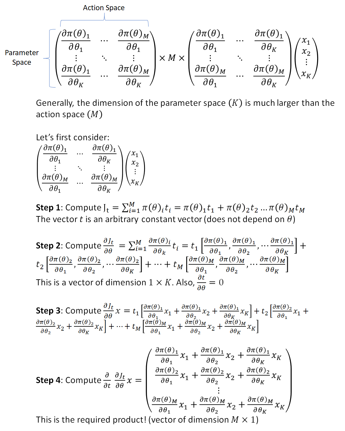
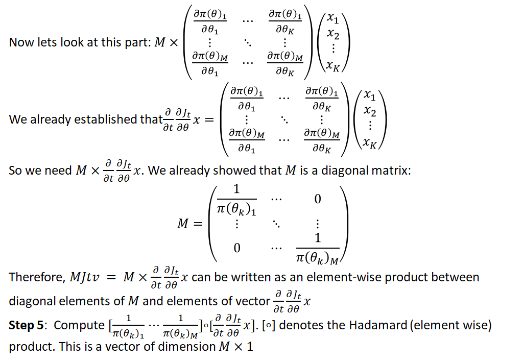
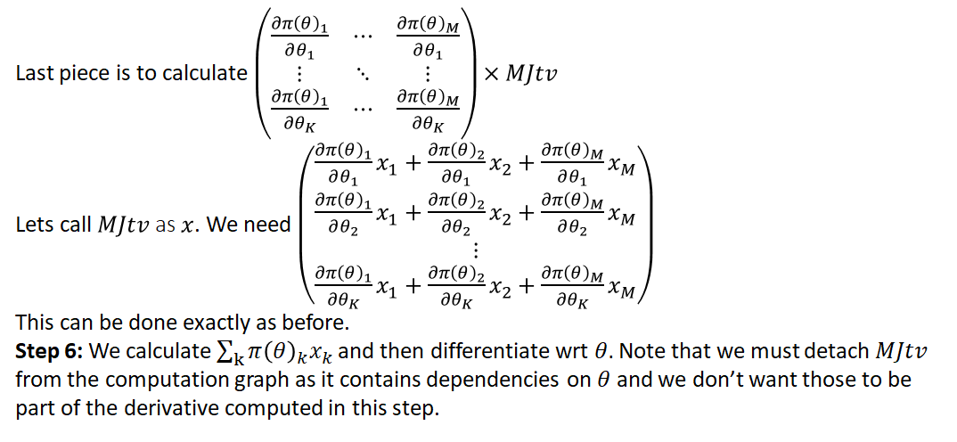
And the code with the steps marked is shown below:

def Fvp_fim(network, states, v):
    damping = 1e-2
    t_beg = time.process_time()
    M, mu, info = network.get_fim(Variable(states))
    mu = mu.view(-1)
    # M is the second derivative of the KL distance wrt network output (M*M diagonal matrix compressed into a M*1 vector)
    # mu is the network output (M*1 vector)
    t = Variable(ones(mu.size()), requires_grad=True)
    # Step 1
    mu_t = (mu * t).sum()
    # Step 2
    Jt = compute_flat_grad(mu_t, network.parameters(), filter_input_ids=set(), create_graph=True)
    # Step 3
    Jtv = (Jt * Variable(v)).sum()
    # Step 4
    Jv = torch.autograd.grad(Jtv, t, retain_graph=True)[0]
    # Step 5
    MJv = Variable(M * Jv.data)
    # Step 6
    mu_MJv = (MJv * mu).sum()
    JTMJv = compute_flat_grad(mu_MJv, network.parameters(), filter_input_ids=set(), retain_graph=True).data
   # JTMJv /= states.shape[0]

    elapsed_time = time.process_time() - t_beg
    global fim_t
    fim_t += elapsed_time
    return JTMJv + v * damping

def Fvp_fim(network, states, v):

damping = 1e-2

t_beg = time.process_time()

M, mu, info = network.get_fim(Variable(states))

mu = mu.view(-1)

# M is the second derivative of the KL distance wrt network output (M*M diagonal matrix compressed into a M*1 vector)

# mu is the network output (M*1 vector)

t = Variable(ones(mu.size()), requires_grad=True)

# Step 1

mu_t = (mu * t).sum()

# Step 2

Jt = compute_flat_grad(mu_t, network.parameters(), filter_input_ids=set(), create_graph=True)

# Step 3

Jtv = (Jt * Variable(v)).sum()

# Step 4

Jv = torch.autograd.grad(Jtv, t, retain_graph=True)[0]

# Step 5

MJv = Variable(M * Jv.data)

# Step 6

mu_MJv = (MJv * mu).sum()

JTMJv = compute_flat_grad(mu_MJv, network.parameters(), filter_input_ids=set(), retain_graph=True).data

# JTMJv /= states.shape[0]

elapsed_time = time.process_time() - t_beg

global fim_t

fim_t += elapsed_time

return JTMJv + v * damping

This method turns out to be about 20% faster than the direct method. This is largely because we are calculating the derivatives of the actions with respect to the network parameters instead of with respect to the KL distance, which is a complex function of the actions. This is a good example of how doing some math in advance yields decent speed-ups over relying on software to do all the derivative calculation.

That’s it! Hope this post will help you with understanding the implementation of TRPO. I welcome your comments/feedback.

Sybil
June 19, 2018 at 9:04 am

i have a question about solving the differentiating wrt s of equation (9) and setting to 0, why the search direction is given by Hs=g? where is lambda? Is g = 1/(lambda)*g?
thank you a lot!

- ankur6ue
  June 20, 2018 at 3:45 pm
  
  Lambda is a scalar, so it doesn’t affect the search direction vector. The size of the search vector is computed in the next step. Makes sense?
  
  - Sybil
    June 22, 2018 at 12:04 am
    
    yes, I understand that. Thanks for your reply!
    
Cheol
November 30, 2018 at 5:14 am

I have a question. Why we need v * damping this part in last return JTMJv + v * damping?
I think just JTMJv is answer.

cheol
November 30, 2018 at 5:16 am

I have one question. why we need damping? I think just JTMJv is ok. why we return JTMJv + v * damping like this?

- ankur6ue
  November 30, 2018 at 4:00 pm
  
  That is just a damping technique used in conjugate gradient methods to make it more stable. See page 3 of this reference: http://www2.maths.lth.se/vision/publdb/reports/pdf/byrod-eccv-10.pdf
  
inexx
October 17, 2019 at 4:10 am

After Eq. 9, why “Differentiating wrt s” won’t lead to “∂(H)/∂(s)”? H and s are both related to θ.

- ankur6ue
  October 17, 2019 at 2:48 pm
  
  yes, but we are differentiating wrt s, not theta. Derivative of g(x)f(x) wrt g(x) = f(x)

Telesens

Efficiently Computing the Fisher Vector Product in TRPO

8 Comments

Leave a Reply Cancel reply